
You type “compare my portfolio to S&P 500” into Google because you want one honest answer: am I beating the index, or would I have been better off just buying it?
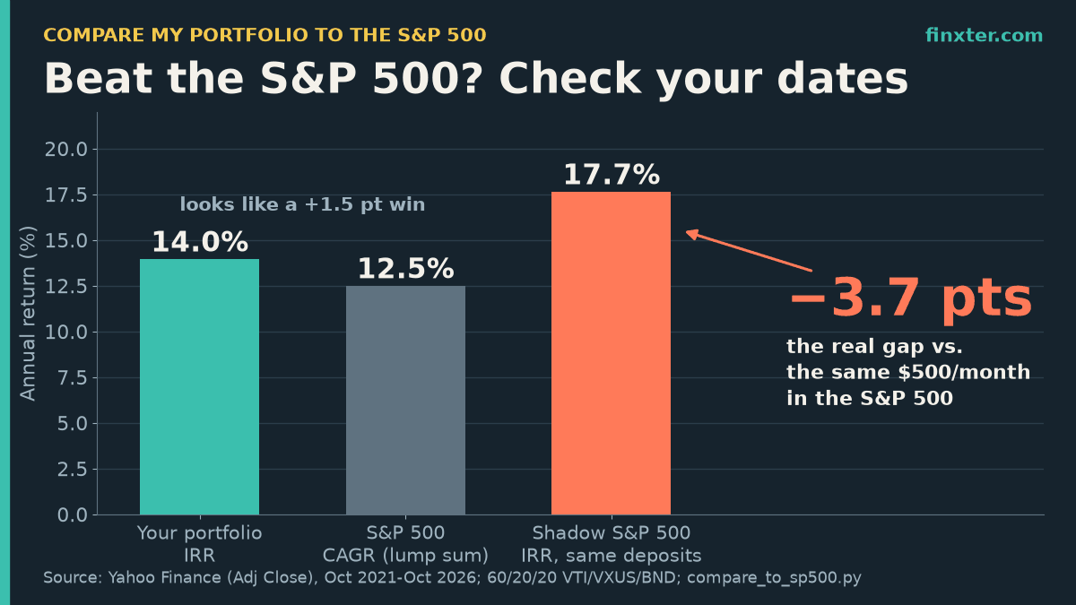
The catch: the two most common ways people run that comparison give the wrong answer. I tested both on five years of real price data, from October 22, 2021 to October 22, 2026, using Yahoo Finance closes and a short pandas script. In the worked example below, a portfolio that looks 1.5 points ahead of the S&P 500 is really 3.7 points a year behind it.
Below you’ll find the three traps, the fix (a “shadow S&P 500” that buys the index with your exact deposits on your exact dates), and a Python script you can point at your own trades.
One side note for readers who write about money: once you’ve run this analysis, you already have the outline of a useful investing guide or newsletter lead magnet. ImagineYourBook is an AI book-writing tool that turns a prompt or your notes into a ~10,000-word draft with Word and EPUB export, so your findings can become a short ebook you then fact-check and edit.
TL;DR
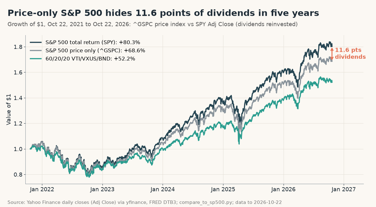
- The price-only S&P 500 rose 68.6% in five years; with dividends (SPY) it rose 80.3%. Compare against total return or you gift yourself 11.6 points.
- $500 a month into a 60/20/20 portfolio earned a 14.0% IRR, which looks 1.5 points ahead of the S&P 500’s 12.5% CAGR.
- A shadow S&P 500 (same dollars, same dates) earned 17.7%: the real gap is −3.7 points a year, or $4,139.
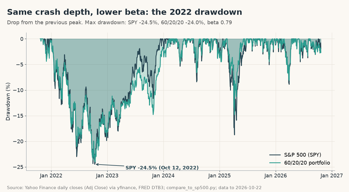
- Risk didn’t rescue it: max drawdown −24.0% vs −24.5%, Sharpe 0.40 vs 0.55.
- Copy the Python script below to run the shadow benchmark on your own trades.
The setup: one example portfolio, five real years
To keep the numbers concrete, I used an example three-fund portfolio. These weights are an assumption for illustration, not a recommendation:
- 60% VTI (US total stock market)
- 20% VXUS (international stocks)
- 20% BND (US bonds)
The benchmark is SPY, an S&P 500 ETF, using Yahoo’s Adjusted Close. Yahoo documents that adjusted close is “the closing price after adjustments for all applicable splits and dividend distributions”, so it behaves like a dividends-reinvested total-return series. For the risk-free rate in the Sharpe ratio, I used the daily 3-month Treasury bill yield (FRED series DTB3), which averaged about 3.8% over the window.
Here is what the script printed:
Period: 2021-10-22 to 2026-10-22 (1255 trading days)
                          Total    CAGR     Vol  Sharpe  Sortino   Max DD
60/20/20 portfolio        52.2%    8.8%   13.9%    0.40     0.58   -24.0%
S&P 500 (SPY, TR)         80.3%   12.5%   17.2%    0.55     0.80   -24.5%
S&P 500 price only        68.6%   11.0%   17.0%    0.48     0.68   -25.4%
Bitcoin                   34.0%    6.0%   51.7%    0.30     0.44   -76.6%
Dividend gap (SPY TR - price index): +11.6% points
Beta vs SPY: 0.79, correlation: 0.98; portfolio max DD on 2022-10-14, SPY on 2022-10-12
$500/month x 61 = $30,500 deposited
  portfolio $43,385 (gain/deposits 42.2%, IRR 14.0%)
  shadow SPY $47,523 (gain/deposits 55.8%, IRR 17.7%)
| Lump sum, Oct 22 2021 to Oct 22 2026 | Total return | CAGR | Volatility | Sharpe | Sortino | Max drawdown |
|---|---|---|---|---|---|---|
| 60/20/20 VTI/VXUS/BND | +52.2% | 8.8% | 13.9% | 0.40 | 0.58 | −24.0% |
| S&P 500 total return (SPY) | +80.3% | 12.5% | 17.2% | 0.55 | 0.80 | −24.5% |
| S&P 500 price only (^GSPC) | +68.6% | 11.0% | 17.0% | 0.48 | 0.68 | −25.4% |
| Bitcoin (BTC-USD) | +34.0% | 6.0% | 51.7% | 0.30 | 0.44 | −76.6% |
Trap 1: comparing against the price-only S&P 500
The number most people Google is the S&P 500 index level (ticker ^GSPC). It ignores dividends.
Over these five years, the price index rose 68.6%. SPY with dividends reinvested rose 80.3%. That is an 11.6-point gap, and it’s almost entirely dividends (SPY’s small fund fee is already netted out of its adjusted close, so the true index-with-dividends gap is slightly larger).
If your brokerage statement counts your dividends but you compare it with the bare index level, you hand yourself 11.6 free points. Always benchmark against a total-return series.
Trap 2: comparing your money-weighted return to the index’s lump-sum return
Most real investors don’t drop one lump sum on day one. They add money every month. So let’s assume $500 on the first trading day of every month, split 60/20/20, for 61 months. That’s $30,500 deposited.
By October 22, 2026, the portfolio was worth $43,385. Its internal rate of return (IRR, a money-weighted return that accounts for when each dollar went in) was 14.0% a year.
Now the common mistake: you look up “S&P 500 five-year annualized return”, find something like SPY’s 12.5% CAGR from our table, and conclude you won by 1.5 points.
But that 12.5% belongs to a single lump sum invested in October 2021, right before the 2022 bear market. Your monthly deposits bought a lot of cheap shares during that drop, which is why your money-weighted figure looks so good. The comparison mixes two different cash-flow patterns. Wikipedia’s time-weighted return article walks through exactly this “problem of external flows”: deposits and withdrawals distort a naive return.
The fix: a shadow S&P 500
Give the S&P 500 the same deal you got. Every time you bought, pretend you bought the same dollar amount of SPY on the same day. Then compare ending values and IRRs.
The shadow S&P 500 ended at $47,523, an IRR of 17.7% a year. Your real gap is −3.7 points a year, or $4,139 on $30,500 of deposits. The fake +1.5-point win was really a 3.7-point loss.
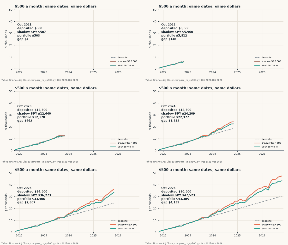
The animation shows the gap opening up month by month: both lines got the same 61 deposits, so the only difference is what the money bought.
Trap 3: ignoring risk (and why “lower risk” didn’t help here)
Return alone isn’t the whole story. A portfolio with 20% bonds should be steadier than 100% stocks, so a fair comparison also looks at risk.
- Volatility: 13.9% for the portfolio vs 17.2% for SPY.
- Beta vs SPY: 0.79, correlation 0.98. The portfolio moved with the market, just a bit less.
- Max drawdown: −24.0% vs −24.5% for SPY, both bottoming in mid-October 2022.
- Sharpe ratio: 0.40 vs 0.55. Sortino: 0.58 vs 0.80.
That drawdown result surprised me. The bonds barely cushioned the crash because BND itself fell 13.1% in calendar 2022 in this data, and VXUS fell 16.1%. So in this particular window the portfolio had nearly the same worst drop and a lower return. Even risk-adjusted, SPY won.
Treat that as a statement about this five-year window, not a law. William Sharpe’s own 1994 paper on the Sharpe ratio separates the ex post (historic) ratio from the ex ante (expected) one. What we computed is ex post: a description of this sample, not a promise about the next five years.
For completeness, the script also runs Bitcoin over the same trading days: +34.0% total with a −76.6% max drawdown. The October 2021 start date sits close to a peak, which shows how much your start date shapes any “vs. benchmark” claim.
The napkin math: why a 3.7-point gap matters more than it sounds
Five years in, the gap is “only” $4,139. Compounding turns that into real money. Assumptions (not forecasts): $500 a month for 20 years, a constant 7% baseline return, and a gap that stays the same every year.
| Annual return (assumed) | Deposits | Value after 20 years | Behind the 10.7% investor |
|---|---|---|---|
| 7.0% (baseline) | $120,000 | $255,203 | $138,231 |
| 8.0% (+1.0 pts) | $120,000 | $286,330 | $107,104 |
| 9.0% (+2.0 pts) | $120,000 | $321,728 | $71,706 |
| 10.7% (+3.7 pts) | $120,000 | $393,434 | $0 |
A persistent 3.7-point shortfall on a 7% baseline leaves you about $138,000 (54%) behind after 20 years on the same $120,000 of deposits. That’s why the shadow benchmark is worth the 10 minutes.
The Python script
This is the exact script that produced every number and chart in this post. It needs pandas, numpy and yfinance; save the FRED DTB3 CSV next to it in src/dtb3.csv. If you’re new to time-series tricks in pandas, the Finxter guide on pandas rolling windows pairs well with the drawdown code (value / value.cummax() - 1).
"""Compare a portfolio to the S&P 500 the right way (Finxter, 2026-10-23).
Data: Yahoo Finance daily closes via yfinance (Adj Close = dividends reinvested), FRED DTB3 3-month T-bill."""
import os, numpy as np, pandas as pd
HERE = os.path.dirname(os.path.abspath(__file__))
START, END = "2021-10-22", "2026-10-22"          # five years, last full close before publishing
WEIGHTS = {"VTI": 0.60, "VXUS": 0.20, "BND": 0.20}  # ASSUMPTION: an example three-fund portfolio
MONTHLY = 500                                       # ASSUMPTION: $500 bought on the first trading day of each month

def load():
    p = os.path.join(HERE, "src", "raw_yf.pkl")
    if os.path.exists(p): raw = pd.read_pickle(p)
    else:
        import yfinance as yf
        raw = yf.download(["SPY", "VTI", "VXUS", "BND", "^GSPC", "BTC-USD"], start="2021-10-01", auto_adjust=False, progress=False)
    adj, close = raw["Adj Close"], raw["Close"]
    days = adj["SPY"].dropna().index                      # stock-market trading days only
    adj, close = adj.loc[days].loc[START:END], close.loc[days].loc[START:END]
    adj["BTC-USD"] = raw["Adj Close"]["BTC-USD"].reindex(adj.index)
    rf = pd.read_csv(os.path.join(HERE, "src", "dtb3.csv"), index_col=0, parse_dates=True, na_values=".")["DTB3"]
    rf = rf.reindex(adj.index).ffill() / 100              # annual T-bill yield
    return adj, close, rf

def portfolio_index(adj, weights=WEIGHTS):
    """Buy-and-hold: invest weights once at START, never rebalance. Value of $1."""
    norm = adj[list(weights)] / adj[list(weights)].iloc[0]
    return sum(w * norm[t] for t, w in weights.items())

def stats(value, rf):
    r = value.pct_change().dropna()
    years = (value.index[-1] - value.index[0]).days / 365.25
    total = value.iloc[-1] / value.iloc[0] - 1
    cagr = (1 + total) ** (1 / years) - 1
    excess = r - rf.loc[r.index] / 252
    sharpe = excess.mean() / r.std() * np.sqrt(252)
    downside = np.sqrt((np.minimum(excess, 0) ** 2).mean()) * np.sqrt(252)
    sortino = excess.mean() * 252 / downside
    dd = value / value.cummax() - 1
    return dict(total=total, cagr=cagr, vol=r.std() * np.sqrt(252), sharpe=sharpe, sortino=sortino,
                max_dd=dd.min(), dd_date=dd.idxmin(), drawdown=dd)

def beta(value, bench):
    a, b = value.pct_change().dropna(), bench.pct_change().dropna()
    return a.cov(b) / b.var(), a.corr(b)

def contributions(adj, weights=WEIGHTS, monthly=MONTHLY):
    """Buy $monthly on the first trading day of each month; same dollars, same dates into SPY (the 'shadow S&P 500')."""
    firsts = adj.groupby(adj.index.to_period("M")).head(1).index
    port_sh = {t: 0.0 for t in weights}; spy_sh = 0.0; flows = []
    for d in firsts:
        for t, w in weights.items(): port_sh[t] += monthly * w / adj.at[d, t]
        spy_sh += monthly / adj.at[d, "SPY"]; flows.append((d, -monthly))
    last = adj.index[-1]
    port_val = sum(s * adj.at[last, t] for t, s in port_sh.items()); spy_val = spy_sh * adj.at[last, "SPY"]
    return dict(deposits=monthly * len(firsts), n=len(firsts), port_val=port_val, spy_val=spy_val, flows=flows, last=last)

def xirr(flows, final_date, final_value):
    cf = flows + [(final_date, final_value)]
    t0 = cf[0][0]; ts = np.array([(d - t0).days / 365.25 for d, _ in cf]); v = np.array([x for _, x in cf])
    lo, hi = -0.99, 1.0
    for _ in range(200):
        mid = (lo + hi) / 2
        if (v / (1 + mid) ** ts).sum() > 0: lo = mid
        else: hi = mid
    return mid

def run():
    adj, close, rf = load()
    port = portfolio_index(adj); spy = adj["SPY"] / adj["SPY"].iloc[0]
    gspc = close["^GSPC"] / close["^GSPC"].iloc[0]; btc = adj["BTC-USD"] / adj["BTC-USD"].iloc[0]
    S = {k: stats(v, rf) for k, v in dict(portfolio=port, spy=spy, gspc=gspc, btc=btc).items()}
    b, c = beta(port, spy)
    C = contributions(adj)
    C["port_irr"] = xirr(C["flows"], C["last"], C["port_val"]); C["spy_irr"] = xirr(C["flows"], C["last"], C["spy_val"])
    return dict(adj=adj, close=close, rf=rf, port=port, spy=spy, gspc=gspc, btc=btc, S=S, beta=b, corr=c, C=C)

if __name__ == "__main__":
    R = run(); S, C = R["S"], R["C"]
    print(f"Period: {R['adj'].index[0].date()} to {R['adj'].index[-1].date()} ({len(R['adj'])} trading days)")
    print(f"{'':22}{'Total':>9}{'CAGR':>8}{'Vol':>8}{'Sharpe':>8}{'Sortino':>9}{'Max DD':>9}")
    for k, lab in (("portfolio", "60/20/20 portfolio"), ("spy", "S&P 500 (SPY, TR)"), ("gspc", "S&P 500 price only"), ("btc", "Bitcoin")):
        s = S[k]; print(f"{lab:22}{s['total']:>9.1%}{s['cagr']:>8.1%}{s['vol']:>8.1%}{s['sharpe']:>8.2f}{s['sortino']:>9.2f}{s['max_dd']:>9.1%}")
    print(f"Dividend gap (SPY TR - price index): {S['spy']['total']-S['gspc']['total']:+.1%} points")
    print(f"Beta vs SPY: {R['beta']:.2f}, correlation: {R['corr']:.2f}; portfolio max DD on {S['portfolio']['dd_date'].date()}, SPY on {S['spy']['dd_date'].date()}")
    print(f"${MONTHLY}/month x {C['n']} = ${C['deposits']:,} deposited")
    print(f"  portfolio ${C['port_val']:,.0f} (gain/deposits {C['port_val']/C['deposits']-1:.1%}, IRR {C['port_irr']:.1%})")
    print(f"  shadow SPY ${C['spy_val']:,.0f} (gain/deposits {C['spy_val']/C['deposits']-1:.1%}, IRR {C['spy_irr']:.1%})")

def napkin_fv(annual_rate, years, monthly=MONTHLY):
    """ASSUMPTION-only napkin math: $monthly at the start of each month, constant annual_rate. Not a forecast."""
    m = (1 + annual_rate) ** (1 / 12) - 1
    return sum(monthly * (1 + m) ** (years * 12 - k) for k in range(years * 12))
To use your own trades, replace WEIGHTS and contributions() with your real buy dates and dollar amounts. The shadow logic stays the same: same dollars, same days, into SPY.
The no-code option
If you’d rather not maintain a script, PortfolioTracker24 is a free, private, browser-based stock and ETF tracker that uses the same idea: its “S&P Equivalent” and “BTC Equivalent” figures replay your dated purchases and sale proceeds into the benchmark. Trades stay in your browser (no account, no broker connection), backups are Excel files, and it reports observed Sharpe, Sortino and drawdown. Be aware of its stated limits: you update prices manually, and cash, dividends, tax and FX aren’t modeled. A $39 one-time Windows edition exists for offline use. For a broader comparison, see Finxter’s roundup of free investment portfolio trackers.
Your 5-step checklist
- Use a total-return benchmark (SPY or VOO adjusted close), never the bare ^GSPC level.
- List every deposit and withdrawal with its date and amount.
- Build the shadow S&P 500: buy the benchmark with the same dollars on the same dates.
- Compare like with like: your IRR vs the shadow’s IRR, your ending value vs the shadow’s ending value.
- Add risk: volatility, max drawdown, Sharpe and beta, and say which window you measured.
| Mistake | What it does to the result (this test) | Fix |
|---|---|---|
| Benchmark = price-only ^GSPC | Understates the S&P 500 by 11.6 points over 5 years | Use SPY/VOO adjusted close (total return) |
| Your IRR vs the index’s lump-sum CAGR | Shows a fake +1.5-point win (14.0% vs 12.5%) | Shadow S&P 500: same dollars, same dates (17.7%) |
| Gain divided by deposits vs 5-year index return | Shows a fake 38-point loss (42.2% vs 80.3%) | Compare with the shadow’s 55.8% gain on deposits |
| Return only, no risk | Hides that the bonds barely cut the 2022 drop | Add volatility, max drawdown, Sharpe, beta |
Limitations
- One example portfolio and one five-year window. A different start date can flip the result.
- Taxes, trading costs and FX aren’t modeled. Bitcoin is sampled on stock-market trading days only.
- Yahoo adjusted closes assume dividends are reinvested on the ex-date at that day’s price.
- Nothing here is investment advice.
Want more Python-for-money projects? The KDP royalty calculator in Python applies the same “script the real rules” approach to book income, and buying and holding tech stocks runs a longer buy-and-hold thought experiment.
The takeaway
To compare your portfolio to the S&P 500 honestly, give the index the same deal you got: same dollars, same dates, dividends included. In this five-year test, that one change turned a “+1.5-point win” into a 3.7-point-a-year loss. Run the shadow benchmark once a year, and you’ll know whether your stock picking is earning its keep.
And if your analysis turns into a story worth sharing, say a “What I learned benchmarking my portfolio” guide for your newsletter, you can draft it with ImagineYourBook. The 7-day trial is $0 today with a card required and includes one 10,000-word Small Book; the first $29.99 charge comes after 7 days unless you cancel before day 8. Check the numbers, add your own charts, and publish it as yours.
Sources (checked October 23, 2026): Yahoo Finance: SPY historical data (daily prices via yfinance) · Yahoo Help: what is the adjusted close? · FRED: 3-Month Treasury Bill secondary market rate (DTB3) · yfinance on GitHub · Wikipedia: time-weighted return and the problem of external flows · William F. Sharpe: The Sharpe Ratio (1994) · PortfolioTracker24 (feature claims checked on its site) · ImagineYourBook pricing and FAQ. Script: compare_to_sp500.py (shown above). Not investment advice.