
Sharpe ratio vs Sortino ratio, in one line: both divide your return above cash by risk, but the Sharpe ratio counts all volatility as risk, while the Sortino ratio counts only the months that fell short of your target. Use Sharpe to compare diversified, roughly symmetric portfolios; use Sortino when returns are lopsided; and never compare one fund’s Sharpe with another fund’s Sortino.
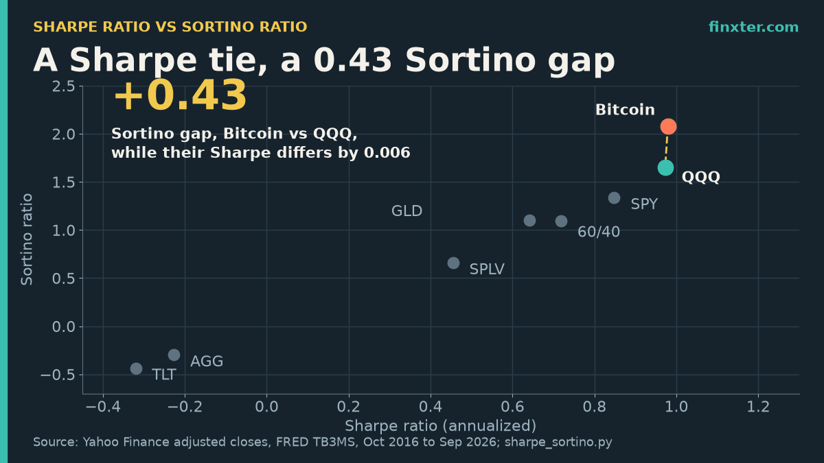
That difference is not academic. On ten years of real monthly data, Bitcoin and the Nasdaq-100 ETF QQQ finished with practically the same Sharpe ratio (0.98 vs 0.97), yet the Sortino ratio rated Bitcoin 2.08 and QQQ 1.65. Same “quality” on one ruler, a 0.43 gap on the other, and Bitcoin still fell −75.6% from peak along the way.
Below are the formulas, the numbers for eight assets, a short pandas script you can run on your own portfolio, and the one Sortino mistake that shows up in a lot of copy-paste code. (If your analysis ends up worth sharing, an AI book tool like ImagineYourBook can turn your notes into a draft investing ebook or lead magnet with Word/EPUB export; more on that at the end.)
TL;DR
- Sharpe divides excess return by all volatility; Sortino divides it by downside deviation only, so it ignores big up months.
- Bitcoin and QQQ tied on Sharpe (0.98 vs 0.97) over Oct 2016 to Sep 2026, but Sortino rated them 2.08 vs 1.65.
- Sortino ran 1.32x to 2.12x the Sharpe ratio across 8 assets, so never compare one fund’s Sharpe with another’s Sortino.
- In 85 rolling 3-year windows the two ratios picked different winners 15 times, always with Sortino favoring Bitcoin, whose max drawdown was −75.6%.
- The popular
returns[returns < 0].std()shortcut is not Sortino: it moved results by about ±9% here. Correct pandas script included.
The two formulas, side by side
Both ratios share the same numerator: the average return minus the risk-free rate (here, the 3-month Treasury bill from FRED’s TB3MS series, which averaged 2.43% a year over the test period).
- Sharpe ratio = average excess return ÷ standard deviation of excess returns. William Sharpe’s own 1994 restatement defines it this way.
- Sortino ratio = average excess return ÷ downside deviation. Downside deviation is the root-mean-square of the shortfalls below the target, where every month at or above the target counts as a shortfall of zero but still counts in the average (Rollinger and Hoffman, “Sortino: A ‘Sharper’ Ratio”).
I use monthly returns and annualize the usual way: multiply the monthly mean by 12 and the monthly deviation by √12.
A worked example: QQQ
For QQQ, October 2016 to September 2026:
- Average excess return: 18.47% a year
- Standard deviation of excess returns: 18.99%
- Downside deviation: 11.21%
So Sharpe = 18.47 ÷ 18.99 = 0.97, and Sortino = 18.47 ÷ 11.21 = 1.65. Same numerator, smaller denominator. That’s why Sortino ratios are almost always bigger than Sharpe ratios for assets that made money, and why “a Sortino of 1.6” and “a Sharpe of 1.0” can describe the same fund.
The data: 8 assets, 120 months
I pulled month-end adjusted closes (dividends reinvested) from Yahoo Finance via yfinance for SPY, QQQ, BTC-USD, GLD, SPLV (low-volatility S&P 500), AGG and TLT, plus a 60/40 SPY/AGG mix rebalanced monthly. The window covers 120 months, October 2016 to September 2026.
| Asset | CAGR | Volatility | Downside dev. | Sharpe | Sortino | Sortino ÷ Sharpe | Skew | Max drawdown |
|---|---|---|---|---|---|---|---|---|
| Bitcoin (BTC-USD) | 63.6% | 74.1% | 34.9% | 0.98 | 2.08 | 2.12x | 0.62 | −75.6% |
| QQQ | 20.9% | 19.0% | 11.2% | 0.97 | 1.65 | 1.69x | −0.21 | −32.6% |
| SPY | 15.2% | 15.3% | 9.7% | 0.85 | 1.34 | 1.58x | −0.44 | −23.9% |
| 60/40 SPY/AGG | 9.6% | 10.2% | 6.7% | 0.72 | 1.10 | 1.53x | −0.42 | −20.0% |
| GLD | 11.7% | 15.5% | 8.9% | 0.64 | 1.10 | 1.72x | 0.11 | −23.8% |
| SPLV | 7.7% | 12.8% | 8.8% | 0.45 | 0.66 | 1.45x | −0.62 | −21.4% |
| AGG | 1.1% | 5.2% | 3.9% | −0.23 | −0.30 | 1.32x | −0.03 | −17.1% |
| TLT | −2.8% | 13.6% | 10.0% | −0.32 | −0.44 | 1.36x | 0.28 | −47.6% |
Three things stand out.
1. The Sortino-to-Sharpe multiple is different for every asset. It ranges from 1.32x (AGG) to 2.12x (Bitcoin). There is no conversion factor, so a fund page quoting Sortino can’t be lined up against another quoting Sharpe.
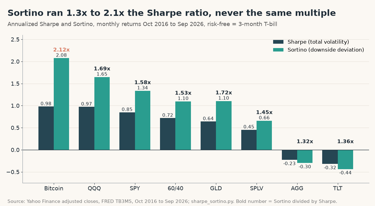
2. Skew drives the multiple. Bitcoin’s monthly returns had a positive skew of 0.62: its big months were up months. Sortino doesn’t penalize those, so its denominator shrinks much more than QQQ’s (skew −0.21) or SPY’s (skew −0.44). Gold, with a mildly positive skew (0.11), got the second-highest multiple, 1.72x.
3. Rankings can flip. By Sharpe, the 60/40 portfolio beats gold, 0.718 to 0.641. By Sortino, gold edges ahead, 1.105 to 1.098. Same data, same months, different winner.
Why Bitcoin and QQQ tie on Sharpe but not on Sortino
Bitcoin’s Sharpe beat QQQ’s by just 0.006. Its Sortino beat QQQ’s by 0.43. Here’s what each ratio is looking at:
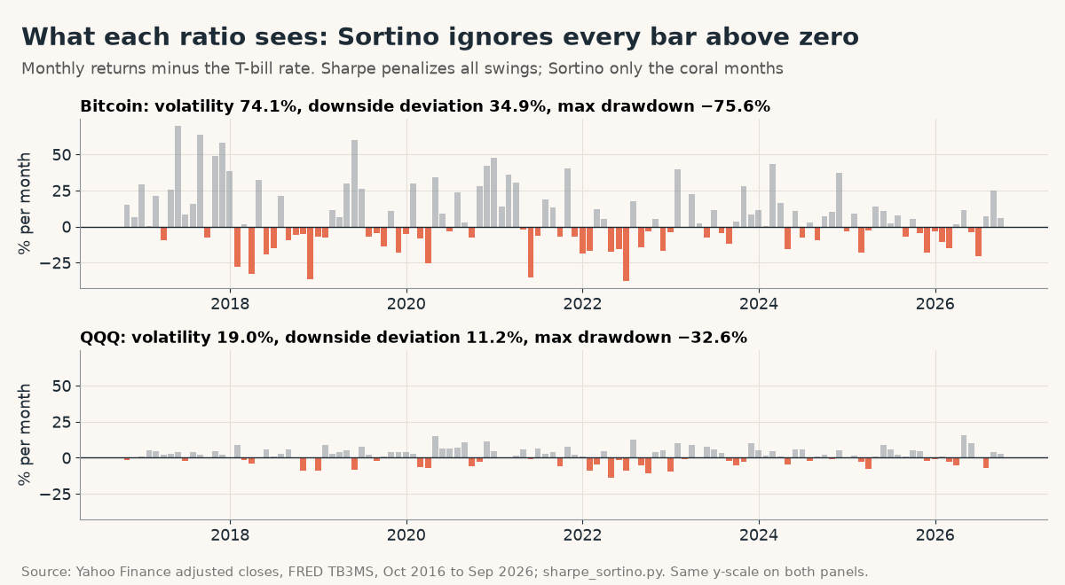
Bitcoin’s volatility (74.1%) is almost four times QQQ’s (19.0%), and much of it comes from huge up months. Sharpe charges Bitcoin for every one of those grey bars. Sortino charges nothing for them, so Bitcoin’s risk measure drops from 74.1% to 34.9%, while QQQ’s drops from 19.0% to 11.2%.
Interesting detail: Bitcoin actually had more months below the T-bill rate, 53 of 120 versus 41 for QQQ. Sortino still likes it more, because downside deviation measures how deep the shortfalls are relative to the return, not how often they happen.
And here’s the catch that neither ratio shows: Bitcoin’s maximum drawdown was −75.6%, QQQ’s −32.6%. A high Sortino is not a promise of shallow losses. It says the typical monthly downside was small relative to the average return, not that the worst stretch was survivable.
Rule: a Sortino ratio tells you the bad months were small on average. It says nothing about how many bad months came in a row. Always print max drawdown next to it.
Does the disagreement last? 85 rolling 3-year windows
One 10-year number can be a fluke, so I recomputed both ratios for Bitcoin and QQQ in every rolling 36-month window (85 windows, ending September 2019 to September 2026).
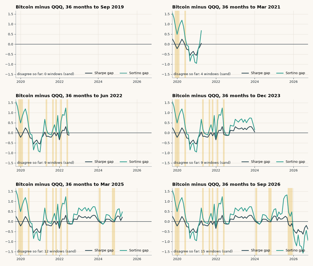
- Bitcoin beat QQQ on Sharpe in 41 of 85 windows.
- Bitcoin beat QQQ on Sortino in 56 of 85 windows.
- The two ratios disagreed on the winner in 15 windows, and in all 15, Sortino picked Bitcoin.
That’s the pattern you’d expect from a positively skewed asset. Sortino isn’t wrong here; it’s answering a different question. If upside surprises are fine with you, Sortino is the more honest score. If you’d have sold in a 75% crash, look at drawdown, not either ratio.
The Sortino mistake in a lot of Python code
A common shortcut is to take returns[returns < 0].std() as the downside risk. That’s not Sortino’s formula. It drops the good months from the average entirely (instead of counting them as zero shortfall) and measures spread around the mean of the bad months instead of distance below the target. The Red Rock paper linked above walks through this exact error.
How much does it matter on real data? With the shortcut, Bitcoin’s Sortino rises from 2.08 to 2.27 (+9.2%), while SPY’s falls from 1.34 to 1.21 (−9.1%). So the shortcut flatters one asset and penalizes another, in the same table.
If you build returns with pandas, Finxter’s guide to pandas pct_change() covers the first step; the script below does the rest correctly.
The Python script
It downloads the prices (or uses a cached copy), builds the 60/40 mix, and prints the full table, both rankings and the rolling comparison. Requirements: pip install yfinance pandas.
"""Sharpe ratio vs Sortino ratio on 10 years of real monthly returns (Oct 2016 to Sep 2026).
Prices: Yahoo Finance adjusted closes (dividends reinvested) via yfinance. Cash rate: FRED TB3MS.
pip install yfinance pandas"""
import numpy as np, pandas as pd

TICKERS = ["SPY", "QQQ", "BTC-USD", "GLD", "SPLV", "AGG", "TLT"]
START, END = "2016-09-30", "2026-09-30"

def load():
    try:  # cached copies used for the article
        adj = pd.read_pickle("src/raw_yf.pkl")["Adj Close"][TICKERS]
        tb = pd.read_csv("src/tb3ms.csv", parse_dates=[0], index_col=0).iloc[:, 0]
    except FileNotFoundError:
        import yfinance as yf
        adj = yf.download(TICKERS, start="2016-01-01", end="2026-10-01", auto_adjust=False, progress=False)["Adj Close"]
        tb = pd.read_csv("https://fred.stlouisfed.org/graph/fredgraph.csv?id=TB3MS", parse_dates=[0], index_col=0).iloc[:, 0]
    r = adj.resample("ME").last().loc[START:END].pct_change().iloc[1:]
    r["60/40"] = 0.6 * r["SPY"] + 0.4 * r["AGG"]          # rebalanced monthly
    tb.index = tb.index + pd.offsets.MonthEnd(0)
    rf = (tb / 100 / 12).reindex(r.index).ffill()           # monthly T-bill return
    return r, rf

def sharpe(r, rf):
    ex = r.sub(rf, axis=0)
    return ex.mean() / ex.std() * np.sqrt(12)

def downside_dev(r, rf):
    """Sortino's target downside deviation: RMS of the shortfalls below the target, over ALL months."""
    ex = r.sub(rf, axis=0)
    return np.sqrt((ex.clip(upper=0) ** 2).mean()) * np.sqrt(12)

def sortino(r, rf):
    return r.sub(rf, axis=0).mean() * 12 / downside_dev(r, rf)

def sortino_wrong(r, rf):
    """Common shortcut: std() of only the negative months. Not Sortino's formula."""
    ex = r.sub(rf, axis=0)
    return ex.mean() * 12 / (ex[ex < 0].std() * np.sqrt(12))

def rolling(r, rf, a="BTC-USD", b="QQQ", months=36):
    """Sharpe and Sortino of two assets in every rolling window (end month as index)."""
    rows = []
    for i in range(months, len(r) + 1):
        w, f = r.iloc[i - months:i][[a, b]], rf.iloc[i - months:i]
        sh, so = sharpe(w, f), sortino(w, f)
        rows.append({"end": w.index[-1], "sh_a": sh[a], "sh_b": sh[b], "so_a": so[a], "so_b": so[b]})
    return pd.DataFrame(rows).set_index("end")

def table(r, rf):
    wealth = (1 + r).cumprod()
    return pd.DataFrame({
        "CAGR": wealth.iloc[-1] ** (12 / len(r)) - 1,
        "Vol": r.std() * np.sqrt(12),
        "DownDev": downside_dev(r, rf),
        "Sharpe": sharpe(r, rf),
        "Sortino": sortino(r, rf),
        "Sortino/Sharpe": sortino(r, rf) / sharpe(r, rf),
        "Skew": r.skew(),
        "MaxDD": (wealth / wealth.cummax() - 1).min(),
        "Shortcut": sortino_wrong(r, rf),
    }).sort_values("Sharpe", ascending=False)

if __name__ == "__main__":
    r, rf = load()
    T = table(r, rf)
    print(f"{len(r)} months, {r.index[0]:%b %Y} to {r.index[-1]:%b %Y}; risk-free = 3-month T-bill (avg {rf.mean()*12:.2%}/yr)")
    print(f"{'':8}{'CAGR':>7}{'Vol':>7}{'DownDev':>8}{'Sharpe':>7}{'Sortino':>8}{'So/Sh':>6}{'Skew':>6}{'MaxDD':>7}{'Shortcut':>9}")
    for k, s in T.iterrows():
        print(f"{k:8}{s.CAGR:>7.1%}{s.Vol:>7.1%}{s.DownDev:>8.1%}{s.Sharpe:>7.2f}{s.Sortino:>8.2f}"
              f"{s['Sortino/Sharpe']:>6.2f}{s.Skew:>6.2f}{s.MaxDD:>7.1%}{s.Shortcut:>9.2f}")
    print("\nRank by Sharpe :", " > ".join(T.index))
    print("Rank by Sortino:", " > ".join(T.sort_values("Sortino", ascending=False).index))
    ex = r["QQQ"] - rf
    print(f"QQQ worked: mean excess {ex.mean()*12:.2%}/yr, std of excess {ex.std()*np.sqrt(12):.2%}, "
          f"downside dev {T.loc['QQQ', 'DownDev']:.2%} -> {ex.mean()*12/(ex.std()*np.sqrt(12)):.2f} and {T.loc['QQQ', 'Sortino']:.2f}")
    g, s = T.loc["GLD"], T.loc["60/40"]
    print(f"GLD vs 60/40: Sharpe {g.Sharpe:.3f} vs {s.Sharpe:.3f}, Sortino {g.Sortino:.3f} vs {s.Sortino:.3f}")
    b, q = T.loc["BTC-USD"], T.loc["QQQ"]
    print(f"BTC vs QQQ: Sharpe gap {b.Sharpe - q.Sharpe:.3f}, Sortino gap {b.Sortino - q.Sortino:.2f}, "
          f"down months {(r['BTC-USD'] < rf).sum()} vs {(r['QQQ'] < rf).sum()} of {len(r)}")
    R = rolling(r, rf)
    print(f"\n{len(R)} rolling 36-month windows (ending {R.index[0]:%b %Y} to {R.index[-1]:%b %Y}):")
    print(f"  BTC beats QQQ on Sharpe in {(R.sh_a > R.sh_b).sum()}, on Sortino in {(R.so_a > R.so_b).sum()}")
    dis = (R.sh_a > R.sh_b) != (R.so_a > R.so_b)
    print(f"  Sharpe and Sortino disagree on the winner in {dis.sum()} windows; Sortino picks BTC in {(dis & (R.so_a > R.so_b)).sum()} of them")
Output, as run for this article:
120 months, Oct 2016 to Sep 2026; risk-free = 3-month T-bill (avg 2.43%/yr)
           CAGR    Vol DownDev Sharpe Sortino So/Sh  Skew  MaxDD Shortcut
BTC-USD   63.6%  74.1%   34.9%   0.98    2.08  2.12  0.62 -75.6%     2.27
QQQ       20.9%  19.0%   11.2%   0.97    1.65  1.69 -0.21 -32.6%     1.55
SPY       15.2%  15.3%    9.7%   0.85    1.34  1.58 -0.44 -23.9%     1.21
60/40      9.6%  10.2%    6.7%   0.72    1.10  1.53 -0.42 -20.0%     1.02
GLD       11.7%  15.5%    8.9%   0.64    1.10  1.72  0.11 -23.8%     1.12
SPLV       7.7%  12.8%    8.8%   0.45    0.66  1.45 -0.62 -21.4%     0.62
AGG        1.1%   5.2%    3.9%  -0.23   -0.30  1.32 -0.03 -17.1%    -0.32
TLT       -2.8%  13.6%   10.0%  -0.32   -0.44  1.36  0.28 -47.6%    -0.54

Rank by Sharpe : BTC-USD > QQQ > SPY > 60/40 > GLD > SPLV > AGG > TLT
Rank by Sortino: BTC-USD > QQQ > SPY > GLD > 60/40 > SPLV > AGG > TLT
QQQ worked: mean excess 18.47%/yr, std of excess 18.99%, downside dev 11.21% -> 0.97 and 1.65
GLD vs 60/40: Sharpe 0.641 vs 0.718, Sortino 1.105 vs 1.098
BTC vs QQQ: Sharpe gap 0.006, Sortino gap 0.43, down months 53 vs 41 of 120

85 rolling 36-month windows (ending Sep 2019 to Sep 2026):
  BTC beats QQQ on Sharpe in 41, on Sortino in 56
  Sharpe and Sortino disagree on the winner in 15 windows; Sortino picks BTC in 15 of them
To use it on your own holdings, replace TICKERS with your funds, or swap r for your portfolio’s own monthly returns. If you want the benchmark side too, the earlier post on how to compare your portfolio to the S&P 500 builds a cash-flow-adjusted S&P 500 twin in Python.
Prefer not to maintain a script? PortfolioTracker24 is a free browser-based tracker that reports observed Sharpe and Sortino ratios and drawdown for your own trades, plus an S&P 500 and Bitcoin comparison. It needs no account or broker connection, keeps data in your browser and backs it up to Excel. Prices are entered manually, and it states that Sharpe and Sortino need a regular return series to be meaningful.
Which one should you use?
| Situation | Use | Why (from this data) |
|---|---|---|
| Comparing index funds or diversified portfolios | Sharpe (Sortino as a check) | SPY, 60/40 and QQQ kept the same order on both ratios |
| Skewed assets: crypto, trend-following, options | Both, side by side | Bitcoin vs QQQ: Sharpe gap 0.006, Sortino gap 0.43 |
| Judging how bad a crash could feel | Max drawdown | Neither ratio flagged Bitcoin’s −75.6% vs QQQ’s −32.6% |
| Comparing numbers from two websites | Only the same ratio, same window and frequency | Sortino ÷ Sharpe ranged 1.32x to 2.12x |
| Writing your own code | Target downside deviation over all periods | The negative-months std() shortcut moved results ±9% |
My rule of thumb after running these numbers:
- Comparing diversified portfolios or index funds? Use Sharpe. Their returns are close enough to symmetric that the extra complexity of Sortino rarely changes the ranking. If you’re tuning a portfolio’s mix, rebalancing matters more; the how often to rebalance backtest found once a year enough on a 40-year 60/40.
- Comparing skewed assets (crypto, trend-following, option-selling, single stocks)? Report both. A big Sortino-over-Sharpe gap tells you the return distribution is lopsided, which is information in itself.
- Always add max drawdown. Neither ratio warned that Bitcoin’s worst fall was 2.3 times deeper than QQQ’s.
- Use one convention throughout: same frequency, same risk-free rate, same window. A monthly Sharpe and a daily Sharpe of the same fund won’t match.
- Be careful with negative ratios. AGG and TLT lost to cash over this decade, and their Sortino ratios (−0.30, −0.44) look “worse” than their Sharpe ratios. With a negative numerator, a smaller denominator makes the number more negative, so don’t read much into the ranking below zero.
Limitations
This is a 10-year sample that includes Bitcoin’s 2017 and 2020-21 booms and a sharp bond sell-off; another decade could rank things differently. Yahoo’s adjusted closes include fund fees and dividends, but not taxes or trading costs. The risk-free rate is the monthly T-bill, used both as the Sharpe baseline and the Sortino target; using 0% as the target would change the Sortino values. Past ratios don’t predict future returns. Nothing here is investment advice.
Takeaway
The Sharpe ratio vs Sortino ratio question has a short answer. Sharpe treats every swing as risk, while Sortino only counts the bad months. That’s why they agree on boring, symmetric portfolios and drift apart on lopsided ones, by 0.43 on the same Sharpe for Bitcoin and QQQ in this test. Calculate both with the right formula, quote them with max drawdown, and you’ll catch what a single number hides.
If you’ve got a spreadsheet full of analysis like this and want to turn it into something shareable, like a short investing guide, a newsletter lead magnet or a family-finance handbook, ImagineYourBook turns a prompt or notes into a complete text draft with a cover, which you then edit and export to Word or EPUB. The trial is $0 for 7 days and includes one 10,000-word Small Book; a card is required, and the Author plan is $29.99 a month after day 7 unless you cancel before day 8. Check the numbers in your draft against your own data before you publish.
Sources (checked October 29, 2026): Yahoo Finance price histories (SPY, QQQ, BTC-USD, GLD, SPLV, AGG, TLT) via yfinance · FRED: 3-Month Treasury Bill rate (TB3MS) · William F. Sharpe, The Sharpe Ratio (1994) · Rollinger & Hoffman, Sortino: A ‘Sharper’ Ratio (Red Rock Capital, PDF) · yfinance on GitHub · PortfolioTracker24 (features as described on its site) · ImagineYourBook pricing and trial terms. Script: sharpe_sortino.py (shown above). Not investment advice.