
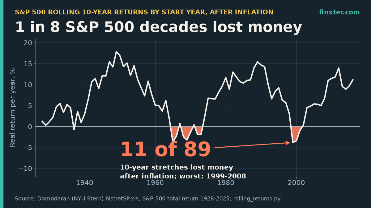
The worst decade to own the S&P 500 wasn’t 1929 to 1938. After inflation, it was 1999 to 2008, when $10,000 turned into $6,781 of today’s buying power. The Great Depression decade actually came out slightly ahead in real terms, because prices fell faster than stocks did.
That’s the twist hiding in S&P 500 rolling 10-year returns. Here is the short answer first: across all 89 rolling 10-year windows from 1928 to 2025 (total return, dividends reinvested), the S&P 500 returned a median 10.96% a year before inflation and 6.71% after it. Before inflation, only 5 of 89 decades lost money. After inflation, 11 of 89 did, about 1 in 8, and most of them weren’t in the 1930s at all.
I computed every rolling window from Aswath Damodaran’s annual S&P 500 dataset (NYU Stern), for 1- to 30-year holding periods, nominal and real. The short Python script and its full output are at the end, so you can rerun it when the 2026 row lands.
TL;DR
- Across 89 rolling 10-year windows (1928-2025), the S&P 500 returned a median 10.96% a year nominal and 6.71% after inflation.
- Before inflation 5 of 89 decades lost money. After inflation 11 of 89 did, about 1 in 8.
- The worst real decade was 1999-2008 (-3.81% a year): $10,000 became $6,781. The Depression decade 1929-1938 was +0.32% real.
- No 20-year window lost money, even after inflation (worst +0.64% a year).
- Top-quartile decades were followed by a median 5.96% real; others by 9.24%. 2016-2025 returned 11.12% real, rank 24 of 89. Python script included.
A side note before the numbers: rolling returns tell you what the market did with your money. The other lever is how much money you add. If you’d like to raise your monthly contribution with a side income, one route is a small catalog of self-published ebooks on Amazon KDP. ImagineYourBook is an AI book-writing tool that turns a prompt or your notes into a complete text draft with a cover, exported as Word and EPUB, with series memory for Book Two and beyond. I run the royalty-to-index-fund math in the closing section.
What “rolling 10-year returns” means
A rolling return looks at every possible holding period of a fixed length, not just the calendar decades. For 10 years, that’s 1928 to 1937, then 1929 to 1938, and so on up to 2016 to 2025: 89 windows from 98 years of data. For each window I compute the annualized total return (CAGR), once in dollars and once after subtracting US inflation.
This beats the usual “the S&P 500 averages 10%” line because it shows the spread you could have lived through, depending on the year you started.
The scoreboard: every holding period from 1 to 30 years
| Holding period | Windows | Negative (nominal) | Negative (real) | Median per year (nominal) | Median per year (real) | Worst real | Best real |
|---|---|---|---|---|---|---|---|
| 1 year | 98 | 26 (26.5%) | 31 (31.6%) | 15.22% | 11.11% | -38.07% (1931) | 53.13% (1954) |
| 3 years | 96 | 15 (15.6%) | 21 (21.9%) | 11.34% | 7.29% | -23.27% (1929-1931) | 28.34% (1954-1956) |
| 5 years | 94 | 11 (11.7%) | 22 (23.4%) | 12.58% | 8.46% | -10.26% (1937-1941) | 25.32% (1995-1999) |
| 10 years | 89 | 5 (5.6%) | 11 (12.4%) | 10.96% | 6.71% | -3.81% (1999-2008) | 17.89% (1949-1958) |
| 15 years | 84 | 1 (1.2%) | 5 (6.0%) | 10.40% | 7.42% | -0.56% (1965-1979) | 15.13% (1985-1999) |
| 20 years | 79 | 0 (0.0%) | 0 (0.0%) | 10.91% | 7.00% | 0.64% (1929-1948) | 13.16% (1980-1999) |
| 30 years | 69 | 0 (0.0%) | 0 (0.0%) | 10.80% | 7.25% | 4.29% (1965-1994) | 10.10% (1932-1961) |
Three things jump out:
- Nominal 10-year losses are rare. Only 5 of 89 windows, and they cluster in two spots: the three windows starting 1928 to 1930, and the two starting 1999 and 2000.
- Inflation doubles the damage. In real terms, 11 of 89 ten-year windows were negative. The real median drops from 10.96% to 6.71% a year.
- 20 years was the line. Not one of the 79 rolling 20-year windows lost money, even after inflation. The worst, 1929 to 1948, still squeezed out 0.64% a year real.
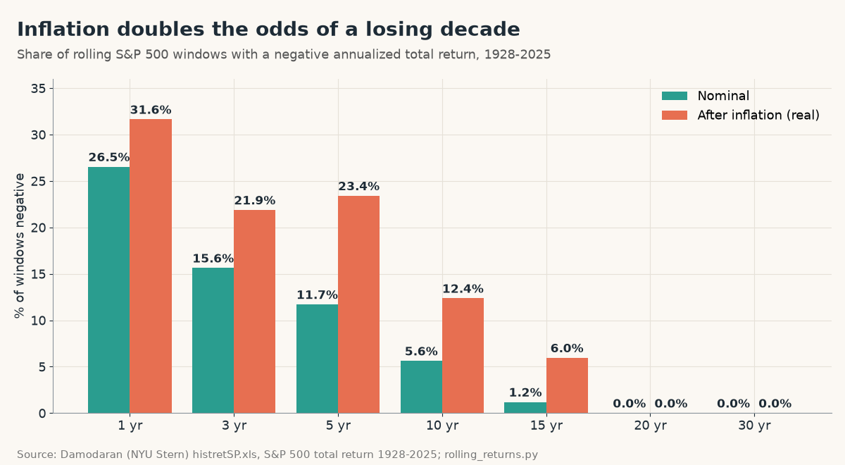
One odd detail in the chart: 5-year windows were more often negative after inflation (23.4%) than 3-year windows (21.9%). That’s the 1970s. Inflation ran hot for years at a time, so it ate entire 5-year stretches while 3-year windows sometimes caught a rally.
Watch the range shrink as you hold longer
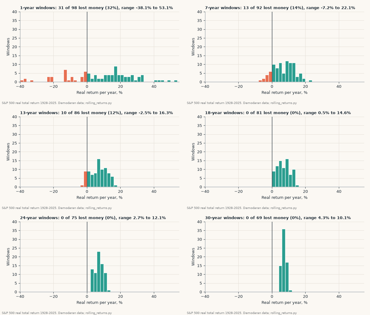
The animation steps through every holding period from 1 to 30 years, using real returns. At 1 year the range runs from -38.07% (1931) to +53.13% (1954). At 10 years it’s -3.81% to +17.89%. At 30 years, it narrows to 4.29% to 10.10% a year, and every single window is positive.
Your average return doesn’t really improve with time; the median real return is 7.00% at 20 years and 7.25% at 30. What improves is the certainty around it.
The 11 decades that lost money after inflation
Here’s the full list, which no “average return” chart shows you:
| 10-year window | Real return per year | What drove it |
|---|---|---|
| 1937 to 1946 | -0.77% | Post-1937 crash, wartime inflation |
| 1965 to 1974 | -3.72% | Late-1960s peak into 1970s inflation |
| 1966 to 1975 | -2.29% | 1970s inflation |
| 1968 to 1977 | -2.44% | 1970s inflation |
| 1969 to 1978 | -3.22% | 1970s inflation |
| 1970 to 1979 | -1.37% | 1970s inflation |
| 1972 to 1981 | -1.92% | 1973-74 bear market, inflation |
| 1973 to 1982 | -1.82% | Inflation 8.68% a year beat a 6.70% nominal return |
| 1999 to 2008 | -3.81% | Dot-com bust + 2008 crash |
| 2000 to 2009 | -3.43% | Dot-com bust + 2008 crash |
| 2001 to 2010 | -0.96% | 2008 crash |
The pattern: inflation, not crashes, made most losing decades. Seven of the 11 come from one stretch, windows starting between 1965 and 1973. From 1973 to 1982, the S&P 500 returned a respectable 6.70% a year in dollars, but inflation averaged 8.68%, so real wealth shrank 1.82% a year.
The Depression is the mirror image. From 1929 to 1938 the index lost 1.67% a year in dollars, its worst nominal decade, but consumer prices fell about 1.98% a year. In real terms that decade returned +0.32% a year. Painful, but not a loss of buying power.
The true worst decade, 1999 to 2008, combined both problems: two crashes (the dot-com bust and 2008) and inflation of about 2.55% a year. Nominal -1.36%, real -3.81%. Put in $10,000 in early 1999 and you had $6,781 of 1999 buying power at the end of 2008.
If you lived through 2008 as an investor, our test of how long it takes the stock market to recover from a crash shows the recovery side of the same story.
What $10,000 did over 10 years: worst, typical, best
Using the real 10-year numbers from the table (inflation-adjusted, so these are in starting-year dollars):
| 10-year window | Real return per year | $10,000 became |
|---|---|---|
| Worst (1999 to 2008) | -3.81% | $6,781 |
| Median of 89 windows | 6.71% | $19,145 |
| Best (1949 to 1958) | 17.89% | $51,852 |
Same index, same 10 years of patience, and a 7.6x gap between the worst and best outcome. That’s why starting dates matter so much in a lump sum, and why the order of returns can make or break a retirement plan (see our sequence of returns risk example).
The uncomfortable part: great decades were followed by weaker ones
Here’s the analysis I couldn’t find in the top results for this keyword. For each 10-year window, I compared its real return to the next 10 years.
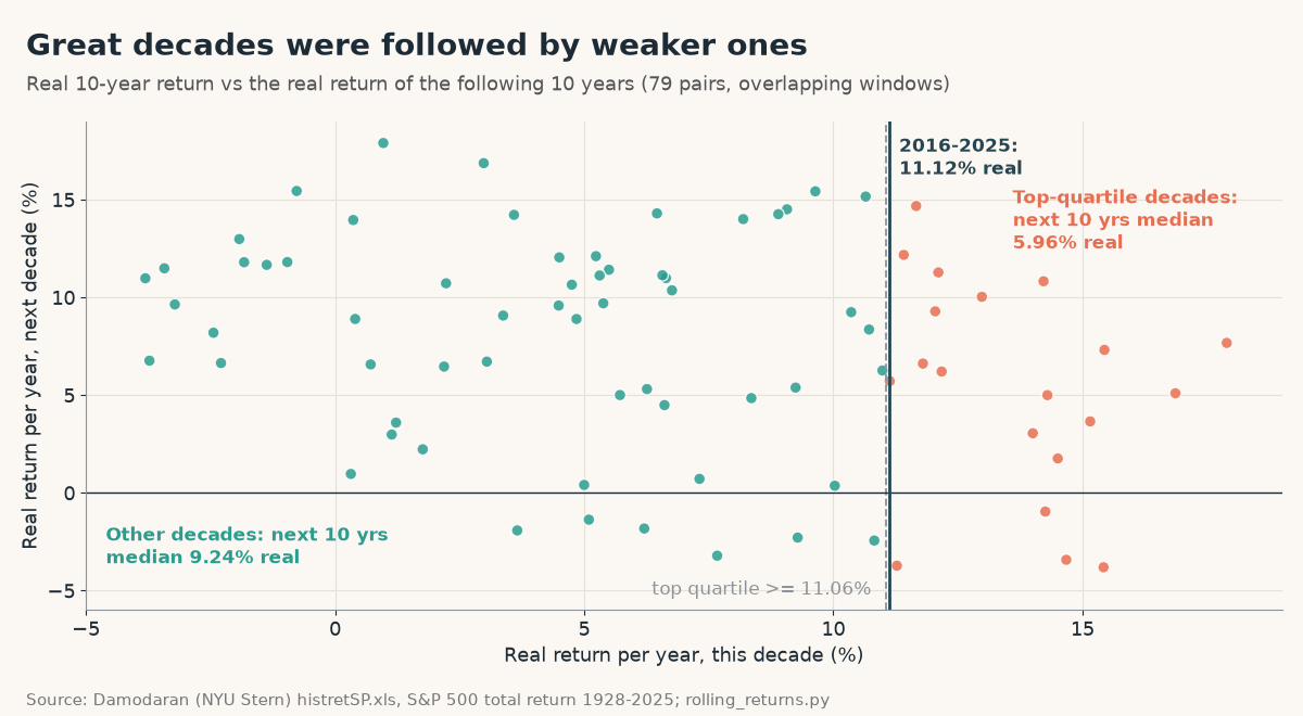
- The 20 decades in the top quartile (real return of 11.06% a year or more) were followed by a median 5.96% real over the next 10 years. The worst follow-up was -3.81% (the 1999 to 2008 decade, which came right after the 1990s boom).
- The other 59 decades were followed by a median 9.24%.
- The correlation between one decade and the next is -0.29: weak, but negative.
Where are we now? The latest complete window, 2016 to 2025, returned 11.12% a year real (14.68% nominal). That ranks 24th of 89 and sits just above the top-quartile line.
Reading this right: after the best quarter of decades, the next 10 years were still positive in the median case (5.96% real), just lower. Lower expected returns are a reason to plan conservatively, not a signal to sell.
Big caveats: the windows overlap heavily, so 79 pairs contain fewer than 10 truly independent decades. This is a pattern, not a forecast, and it says nothing about which year a slowdown would start. Missing the market isn’t the fix either; see what missing the best days in the market costs.
How to use rolling returns in your own plan
- Plan with the real median, not 10%. For a 10- to 30-year plan, 6.71% to 7.25% real is the historical middle. If your plan only works at 10% nominal and ignores inflation, it’s leaning on the good half of history.
- Money you need within 10 years isn’t safe in stocks alone. About 1 in 8 real 10-year windows lost money, and 23.4% of 5-year windows did.
- Contribute on a schedule. Rolling returns describe a single lump sum. Monthly buying spreads your entry points across many windows; our lump sum vs DCA test shows both paths.
- Check your own portfolio’s real dates. Your returns depend on when you bought.
To see how your actual buys compare with the S&P 500, with your real dates and amounts, PortfolioTracker24 is a free, private tracker that runs in your browser: no account, no broker connection, and you keep an Excel backup. For a Python version of that check, see compare my portfolio to the S&P 500.
The Python script
It downloads Damodaran’s spreadsheet once (cached to src/) and prints every number in this article. You need pip install pandas requests xlrd. New to pandas? Start with the Finxter pandas quickstart.
# S&P 500 rolling returns, nominal and after inflation, 1928-2025
# Data: Aswath Damodaran (NYU Stern), histretSP.xls, sheet "Nominal vs Real Data"
import os, requests, numpy as np, pandas as pd

URL = "https://pages.stern.nyu.edu/~adamodar/pc/datasets/histretSP.xls"
FILE = "src/histretSP.xls"

def load():
    if not os.path.exists(FILE):
        os.makedirs("src", exist_ok=True)
        open(FILE, "wb").write(requests.get(URL, headers={"User-Agent": "Mozilla/5.0"}).content)
    df = pd.read_excel(FILE, "Nominal vs Real Data", usecols=[0, 1, 4, 5])
    df.columns = ["year", "nominal", "inflation", "real"]
    df = df[pd.to_numeric(df.year, errors="coerce").notna()].astype(float)
    return df.astype({"year": int}).set_index("year")

def rolling_cagr(r, n):
    """Annualized return of every n-year window, indexed by its last year."""
    growth = (1 + r).rolling(n).apply(np.prod, raw=True)
    return (growth ** (1 / n) - 1).dropna()

if __name__ == "__main__":
    df = load()
    print(f"years {df.index[0]}-{df.index[-1]} ({len(df)})")
    for col in ("nominal", "real"):
        print(f"\n{col.upper()} (total return, dividends reinvested)")
        for n in (1, 3, 5, 10, 15, 20, 30):
            s = rolling_cagr(df[col], n)
            lo, hi = s.idxmin(), s.idxmax()
            print(f"{n:>2}y: {len(s):>2} windows, {(s < 0).sum():>2} negative ({(s < 0).mean():5.1%}), "
                  f"median {s.median():6.2%}, worst {s.min():7.2%} ({lo-n+1}-{lo}), best {s.max():6.2%} ({hi-n+1}-{hi})")
    s = rolling_cagr(df.real, 10)
    print("\nNegative real 10-year windows:", ", ".join(f"{y-9}-{y} {v:.2%}" for y, v in s[s < 0].items()))
    pair = pd.DataFrame({"this": s, "next": s.shift(-10)}).dropna()
    q = pair.this.quantile(0.75)
    top, rest = pair[pair.this >= q], pair[pair.this < q]
    print(f"Latest window 2016-2025: real {s[2025]:.2%}, rank {(s > s[2025]).sum() + 1} of {len(s)}")
    print(f"Top-quartile decades (real >= {q:.2%}, n={len(top)}): next decade median {top.next.median():.2%}, "
          f"worst {top.next.min():.2%}; other decades (n={len(rest)}): next median {rest.next.median():.2%}; "
          f"correlation {pair.corr().iloc[0, 1]:.2f}")
Output (data through 2025):
years 1928-2025 (98)

NOMINAL (total return, dividends reinvested)
 1y: 98 windows, 26 negative (26.5%), median 15.22%, worst -43.84% (1931-1931), best 52.56% (1954-1954)
 3y: 96 windows, 15 negative (15.6%), median 11.34%, worst -27.30% (1930-1932), best 30.85% (1995-1997)
 5y: 94 windows, 11 negative (11.7%), median 12.58%, worst -12.71% (1928-1932), best 28.29% (1995-1999)
10y: 89 windows,  5 negative ( 5.6%), median 10.96%, worst  -1.67% (1929-1938), best 20.11% (1949-1958)
15y: 84 windows,  1 negative ( 1.2%), median 10.40%, worst  -0.20% (1929-1943), best 18.80% (1985-1999)
20y: 79 windows,  0 negative ( 0.0%), median 10.91%, worst   2.37% (1929-1948), best 17.69% (1980-1999)
30y: 69 windows,  0 negative ( 0.0%), median 10.80%, worst   7.97% (1929-1958), best 13.63% (1970-1999)

REAL (total return, dividends reinvested)
 1y: 98 windows, 31 negative (31.6%), median 11.11%, worst -38.07% (1931-1931), best 53.13% (1954-1954)
 3y: 96 windows, 21 negative (21.9%), median  7.29%, worst -23.27% (1929-1931), best 28.34% (1954-1956)
 5y: 94 windows, 22 negative (23.4%), median  8.46%, worst -10.26% (1937-1941), best 25.32% (1995-1999)
10y: 89 windows, 11 negative (12.4%), median  6.71%, worst  -3.81% (1999-2008), best 17.89% (1949-1958)
15y: 84 windows,  5 negative ( 6.0%), median  7.42%, worst  -0.56% (1965-1979), best 15.13% (1985-1999)
20y: 79 windows,  0 negative ( 0.0%), median  7.00%, worst   0.64% (1929-1948), best 13.16% (1980-1999)
30y: 69 windows,  0 negative ( 0.0%), median  7.25%, worst   4.29% (1965-1994), best 10.10% (1932-1961)

Negative real 10-year windows: 1937-1946 -0.77%, 1965-1974 -3.72%, 1966-1975 -2.29%, 1968-1977 -2.44%, 1969-1978 -3.22%, 1970-1979 -1.37%, 1972-1981 -1.92%, 1973-1982 -1.82%, 1999-2008 -3.81%, 2000-2009 -3.43%, 2001-2010 -0.96%
Latest window 2016-2025: real 11.12%, rank 24 of 89
Top-quartile decades (real >= 11.06%, n=20): next decade median 5.96%, worst -3.81%; other decades (n=59): next median 9.24%; correlation -0.29
FAQ
What is the average rolling 10-year return of the S&P 500?
From 1928 to 2025, the median rolling 10-year return was 10.96% a year with dividends reinvested, or 6.71% after inflation, across 89 overlapping windows (Damodaran data).
Has the S&P 500 ever had a negative 10-year return?
Yes. In dollars, 5 of 89 rolling 10-year windows were negative, the worst 1929 to 1938 at -1.67% a year. After inflation, 11 of 89 were negative, the worst 1999 to 2008 at -3.81% a year.
What was the worst 10-year period for the S&P 500?
After inflation, 1999 to 2008: -3.81% a year, so $10,000 shrank to $6,781 in real terms. In nominal dollars the worst was 1929 to 1938 at -1.67% a year.
Has the S&P 500 ever lost money over 20 years?
Not from 1928 to 2025. All 79 rolling 20-year windows were positive, even after inflation. The weakest, 1929 to 1948, returned 0.64% a year real and 2.37% nominal.
What does a strong decade mean for the next 10 years?
Historically, decades in the top quartile (11.06% or more real) were followed by a median 5.96% real over the next 10 years, versus 9.24% after other decades. Windows overlap, so treat it as a pattern, not a forecast.
The takeaway: the market sets the return, you set the contribution
Rolling 10-year returns say the S&P 500’s typical decade grew wealth about 6.71% a year after inflation, with 1 in 8 decades going backward. You can’t pick your decade. You can pick how much you put in.
Here’s the napkin math for that second lever. Amazon KDP pays a 70% ebook royalty on list prices from $2.99 to $9.99, before a small delivery fee. At $4.99, that’s about $3.49 per sale. Assumption, not a typical result: if a few books together sold 30 copies a month, that’s about $104.79 a month before delivery fees. Invest $100 of it every month for 10 years at the median real 10-year return of 6.71%, and you’d have about $17,035 in today’s dollars. Sales are never guaranteed and many books sell far less, so treat this as a scenario to test, not a promise. For your own numbers, try the KDP royalty calculator.
If you want to try that route, ImagineYourBook can turn an idea or your notes into a full text draft with a cover, ready to edit and publish on KDP. The 7-day trial is $0 with a card and includes one 10,000-word book; if you don’t cancel before day 8, the first charge is $24.99 a month. You still do the editing, the fact check and the marketing.
Sources (checked November 16, 2026): Aswath Damodaran (NYU Stern): Historical returns on stocks, bonds and bills, 1928-2025 · histretSP.xls (S&P 500 total return, inflation, real return) · Amazon KDP: eBook Royalties · Finxter: KDP delivery fee · ImagineYourBook pricing and trial terms · PortfolioTracker24. Script: rolling_returns.py (shown above). Past returns don’t predict future returns. Not investment advice.