Gradient Descent in Neural Nets – A Simple Guide to ANN Learning

💡 Gradient Descent: What is it? Where does it come from? And what the heck is it doing in my ANN?

You can scroll through the slides as you watch this video here:

This article aims to present the gradient descent algorithm in a light fashion, familiarizing new Machine Learning enthusiasts with this fundamental technique… and convincing them that it is not rocket science 😉

Gradient descent is a widely known optimization algorithm, broadly used in Machine Learning and several areas of Mathematics.

More specifically, in gradient descent we are trying to find the minimum of a given (differentiable) function defined on an -dimensional Euclidean space ,

💡 General Idea: The process starts by picking up a (possibly random) point in the optimization space and following the direction opposed to the gradient of the function at that point. After moving a bit towards the specified direction, you repeat the process starting from the resulting new point. 

Next, we explain why gradients are the (opposite of the) right direction to follow, and do it through a small caveat: gradients do not exist…

Why Gradients?

…naturally. Gradients are ad-hoc objects resulting from two other entities: the differential of the function and the underlying metric of the Euclidean space.

It exists as a consequence of the linearity of the derivative.

That is, for every pair of vectors v and w, the differential in the direction of v+w can be computed as the sum of the differential of v and the differential of w:

Another linear object is the inner product with a fixed vector: fixing a vector , one has that

Now, the famous Riez Representation Theorem connects the two linear objects above by guaranteeing the existence of a unique vector whose inner product coincides with computing the differential (guess which vector it is):

and here it is the gradient.

Another expression for the inner product above uses the angle between and v:

By inspecting it, we conclude that the differential of f at p realizes its maximum in the direction of and maximally decreases towards .

That is to say, the negative of the gradient points towards the direction of greatest reduction of the function. Therefore, flowing along the negative gradient seems a great path to find a (local) minimum.

Besides, an exercise using the unicity part of the Riez’s Theorem shows that the Euclidean coordinates of the vector representing is computed through the well-known expression:

Nevertheless, back to our caveat, this expression does not generalize to other coordinate systems as the expressions in cylindrical and spherical coordinates show… and don’t think you will be safe from non-Euclidean geometry for long 😉

How Does Gradient Descent Relate to Machine Learning?

Gradient descent plays a central role in Machine Learning, being the algorithm of choice to minimize the cost function.

The common Machine Learning task is to use plotted data to predict the value of new data entries.

Precisely, given a set of labeled data, that is, tuples of features and target values, the algorithm tries to fit a candidate modeling function to it. The better candidate is selected as the one evaluating the minimal cost function among all candidates, and that is where the gradient descent comes into play.

To picture this, let us take a look at the data in Housing Prices Competition for Kaggle Learn Users, especially the relation between Sale’s Price and Lot Area:

Figure 1: Scatter plot of the sale’s price of a house versus its Lot Area.

By the way, you can check out our tutorial on how we created all the plots in this tutorial:

👉 Recommended Tutorial: Plotting Vector Fields and Gradients for ANN Gradient Descent

The simplest model used in Machine Learning is called linear regression, where a line is fitted through the plotted points. Such a procedure consists in choosing two parameters, the bias and the angular coefficient of the line, respectively b and a below:

A typical cost function for this task is the Mean Square Error (MSE), which is directly computed on the parameters a and b:

Here stand for the Lot Area and the Sale’s Price of the i-th entry and n is the number of points plotted.

When the MSE is applied to the linear regression case, the resulting function lies within the special class of convex functions.

These have the nice property of having a unique minimum that is achieved through gradient descent independent of the point you start (as long as your learning rate is not high). 

Unfortunately the general case does lead us to such a simplified scenario, and the cost function might have several local minima. This is a typical situation in Artificial Neural Networks. 

Feedforward Neural Networks and Their Challenges 

A more complex family of candidates is given by Neural Networks. Even so, in the specific case of Feedforward Neural Networks, a rephrasing of the last statement is really enlightening: a FNN is exactly (not more, nor less than) another family of candidate functions.

Instead of using a line to reveal a pattern in the scattered plot, one uses a more elaborate family of functions. In particular, the gradient descent works out of the box.

In the case of FNN’s, the candidate function is given by a composition of simpler functions:

while:

• stands for the vector of the given features;
• is the total number of layers chosen in the architecture of the Network;
• is the matrix consisting of the weights connecting the (l-1)-th layer with the l-th layer;
• is the activation function of the l-th layer.

Activation functions are theoretically arbitrary, but are usually chosen as functions whose derivative can be easily calculated.

Due to the linearity of , and choice of simple activation functions, the gradient of g can be efficiently computed using the chain rule.

Therefore, the gradient of the cost function becomes a feasible object by using the more general expression of the former:

Note that x is a given data entry and every other parameter described above is fixed a priori. Hence, J is represented as a function depending solely on the weights .

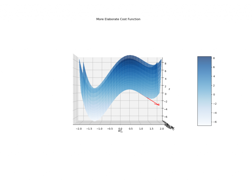
The gradient descent makes itself present once more being a reasonable way to find local minima. In this case, though, J is usually much more complicated and a situation similar to the one below might happen:

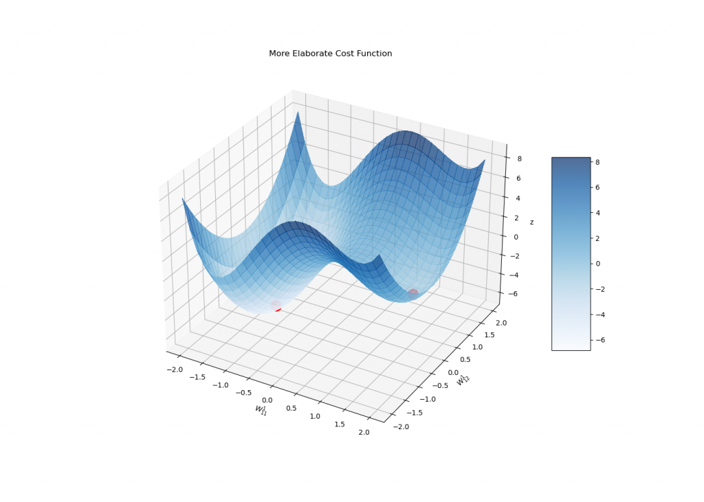
Observe how the gradient leads us to the wrong minima if not initialized carefully: 

Maybe a side view? 

In fact, the stopping condition of the gradient descent is to reach a critical point of J, i.e., a point whose gradient is zero.

In this sense, the algorithm itself will never discriminate between reaching a global minimum or even a saddle point (which is not even a local minima!), although the gradient flow is very unstable near other types of critical points (and usually do not converge to them).

In any case, it might be a reasonable idea to eventually initialize the gradient descent in a few sparsely distributed random points in order to reach lower cost values.

Concluding Remarks

Gradient descent is a robust optimization method, widely used in Machine Learning algorithms.

Although Neural Networks’ candidates present elaborate derivatives, do not panic: your job in NN is to have fun choosing the right architecture, starting point, learning rate and some other stuff. The gradients and core mathematical calculations are all done by your favorite ML package.

For more details on FNN, Wikipedia offers a well-tailored article on Backpropagation.

And if you didn’t buy yet the importance of using gradient descent, take a few minutes to compare it to a brute force method, at the section ‘Curse of dimensionality’ in this nice article.

The weights on Neural Networks are usually organized as tensors (TensorFlow = Tensor + (gradient) Flow, got it?). You can learn more about them in Aaron’s great article. 

Happy coding!