
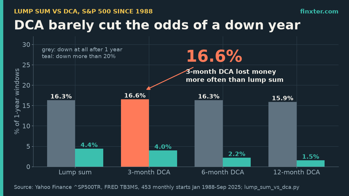
Dollar-cost averaging is sold as protection against a bad first year. On the S&P 500 since 1988, the popular 3-month DCA was still down after one year in 16.6% of start months, slightly more often than putting the whole lump sum in on day one (16.3%).
That is the non-obvious part of the lump sum vs DCA S&P 500 question, and it changes what DCA is actually for. The short answer first: across 453 rolling start months (January 1988 to September 2025, dividends reinvested, idle cash earning T-bill interest), investing the lump sum at once beat DCA 64.7% of the time against a 3-month plan and 77.7% of the time against a 12-month plan. DCA did not lower your odds of a losing year in any meaningful way. What a long DCA did buy was a thinner tail: a 12-month plan cut the share of years that lost more than 20% from 4.4% to 1.5%. The median price of that was $4,677 per $100,000.
TL;DR
- Lump sum beat DCA on the S&P 500 in 64.7% (3-month plan) to 77.7% (12-month plan) of 453 start months since 1988.
- DCA did not cut the odds of a losing year: 16.3% for lump sum vs 16.6%, 16.3% and 15.9% for 3-, 6- and 12-month DCA.
- A 12-month DCA did shrink the tail: years losing more than 20% fell from 4.4% to 1.5%, worst year −33.3% instead of −43.3%.
- The price: a median $4,677 per $100,000 after one year, about $16,915 by year 20 at an assumed 7%.
- Python script included: swap the ticker or the DCA length and rerun.
The numbers below come from a short Python script you can run yourself (full code further down). It builds on the shadow-benchmark idea from how to compare your portfolio to the S&P 500 the right way: same index, same dollars, only the timing changes.
A side note for readers who turn analyses like this into something publishable: a clean backtest plus your own rules is the skeleton of a short investing ebook or a newsletter lead magnet. If that’s your next step, ImagineYourBook is the AI book-writing tool I’d start with: it turns a prompt or your notes into a complete 10,000-word draft with its own cover, and paid plans export Word and EPUB for editing. You still check every number yourself, which you already do.
The setup: what “lump sum” and “DCA” mean here
Imagine $100,000 lands in your account at a month-end: a bonus, an inheritance, the sale of a business.
- Lump sum: buy the S&P 500 total-return index with all of it that day.
- DCA (dollar-cost averaging): invest 1/3, 1/6 or 1/12 of it at each month-end, starting that day. The cash still waiting earns the 3-month T-bill rate (FRED series TB3MS), so DCA is not handicapped by idle cash earning zero.
- Scorecard: compare both after exactly 12 months, the same horizon Vanguard’s 2023 study uses.
Data: Yahoo Finance’s ^SP500TR, the S&P 500 with dividends reinvested, month-end closes from January 1988 to September 2026. That gives 453 start months, each with a full year to measure. One useful detail: once the DCA plan is fully invested, both portfolios hold the same index, so whatever percentage gap exists at month 12 stays locked in for good. Measuring at one year is not a short-term trick. It is the permanent result.
Result 1: lump sum wins most of the time, and the gap grows with DCA length
| Strategy | Lump sum beat it | Median lump-sum edge | Down after 1 year | Down >20% | Worst year |
|---|---|---|---|---|---|
| Lump sum (all on day 1) | n/a | n/a | 16.3% | 4.4% | −43.3% |
| 3-month DCA | 64.7% | 1.08% | 16.6% | 4.0% | −43.9% |
| 6-month DCA | 68.9% | 2.20% | 16.3% | 2.2% | −43.2% |
| 12-month DCA | 77.7% | 4.24% | 15.9% | 1.5% | −33.3% |
The 3-month row is the one Vanguard uses as its base case. Vanguard found that lump sum beat cost averaging 68% of the time on the MSCI World index (1976–2022), with a range of 61.6% to 73.7% across markets and split lengths. My 64.7% on the S&P 500 sits inside that range, which is a good sanity check for the script.
The pattern is simple: every extra month in cash is a month without the equity risk premium. Stretch the DCA from 3 to 12 months and lump sum’s win rate climbs from 64.7% to 77.7%, while the median edge grows from 1.08% to 4.24%.
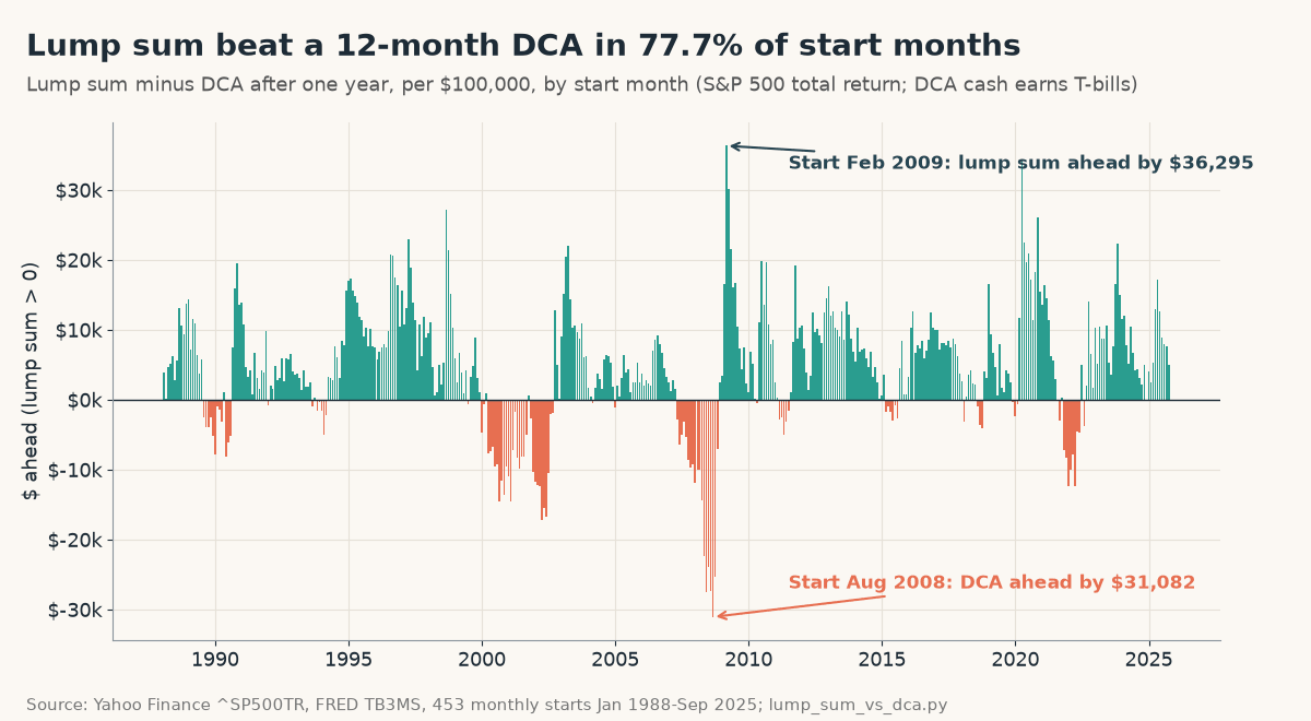
The chart also shows that DCA’s wins are not rare flukes. They cluster in exactly the years you remember: 2000–2002 and 2007–2008. Start a 12-month DCA in August 2008 and your $100,000 was worth $112,829 a year later, while the lump sum sat at $81,747, a $31,082 difference. Start in February 2009, near the bottom, and the lump sum was ahead by $36,295.
On average the two sides win by similar amounts: $7,895 per $100,000 when lump sum wins, $7,190 when DCA wins. So the decision is about how often, and lump sum wins about three times out of four over 12 months.
Result 2: DCA does not lower the odds of a losing year
This is the convention-breaking part. The usual pitch for DCA is “you won’t lose money if the market drops right after you invest.” Count the losing years:
- Lump sum: down after one year in 74 of 453 windows (16.3%).
- 3-month DCA: down in 75 (16.6%).
- 6-month DCA: down in 74 (16.3%).
- 12-month DCA: down in 72 (15.9%).
That’s a difference of one or two windows out of 453, which is noise. The reason is simple once you look at it: a bear market that lasts a year (2001, 2008) pulls down money invested in month 3 almost as much as money invested in month 1. And in flat years, DCA can buy after a small rise and end slightly below zero while the lump sum ends slightly above it.
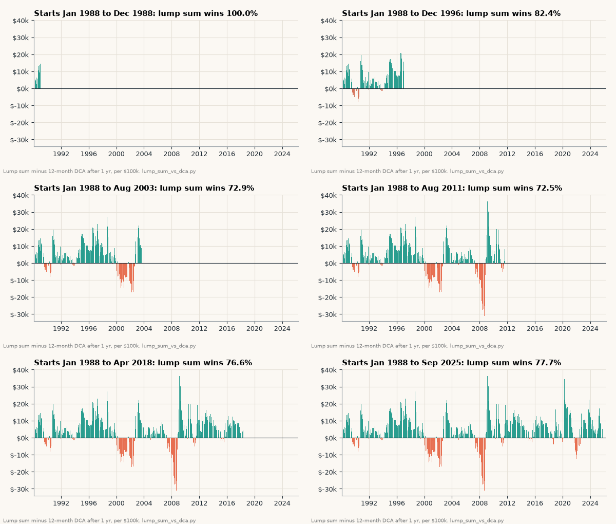
The animation builds the 12-month comparison start month by start month. Watch the running win rate: it climbs to about 85% by the end of the 1990s, slides to about 71% by 2002 as the dot-com and 2008 starts pile up (lump sum won only 57.5% of the 2000s starts), then recovers to 77.7%.
Result 3: what DCA actually buys is a thinner tail
If DCA doesn’t prevent losing years, what does it do? It makes the bad losing years less bad, but only if you spread it out long enough.
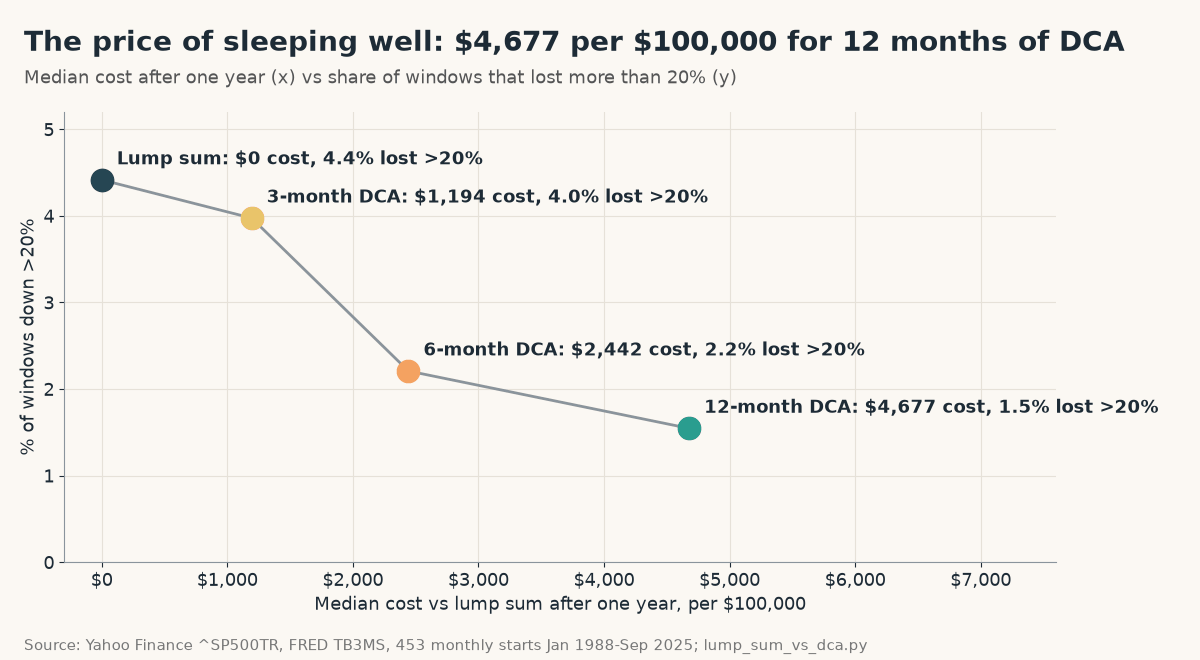
- The worst lump-sum year (start February 2008) lost 43.3%. The worst 12-month DCA year lost 33.3%.
- Lump sum lost more than 20% in 4.4% of windows (20 of 453). The 12-month DCA did so in 1.5% (7 windows).
- A 3-month DCA barely moved the tail: 4.0%, and its worst year (−43.9%) was no better than the lump sum’s.
So think of DCA as an insurance policy against the one-in-twenty disaster year, with a premium you pay in the other nineteen. The premium is not small.
The compounding napkin math: what the premium costs over 20 years
The median 12-month DCA trailed the lump sum by $4,677 per $100,000 after one year. Because both portfolios are fully invested from then on, that gap compounds along with everything else.
| Plan | Median cost after 1 year | Cost by year 20 (assumed 7%/yr) | Years down >20% |
|---|---|---|---|
| Lump sum | $0 | $0 | 4.4% |
| 3-month DCA | $1,194 | $4,317 | 4.0% |
| 6-month DCA | $2,442 | $8,831 | 2.2% |
| 12-month DCA | $4,677 | $16,915 | 1.5% |
The two right-hand columns rest on an assumption, not data: both portfolios then grow at 7% a year with no taxes, fees or new deposits. Under that assumption the median 12-month DCA costs about $16,915 by year 20. The 3-month version costs about $4,317. Neither is a forecast. The point is the ratio: you pay roughly four times more for the 12-month plan, and it’s the only one that meaningfully cut the tail.
If you’re doing similar planning for a fixed goal, the same compounding logic is in this Python plan for having $70k for a kid at 21.
The Python script
It uses only pandas and yfinance. Month-end resampling is one line (see Finxter’s pandas resample() guide if that’s new). Swap ^SP500TR for any ticker, or change n to test a 9-month plan.
"""Lump sum vs DCA on the S&P 500 (total return), every rolling start month since 1988.
Data: Yahoo Finance ^SP500TR (dividends reinvested) month-end closes; FRED TB3MS (3-month T-bill) for idle DCA cash.
pip install yfinance pandas"""
import pandas as pd

def load(end="2026-09-30"):
    try:  # cached copies used for the article
        px = pd.read_pickle("src/SP500TR.pkl")["Close"].squeeze()
        tb = pd.read_csv("src/tb3ms.csv", parse_dates=[0], index_col=0)["TB3MS"]
    except FileNotFoundError:
        import yfinance as yf
        px = yf.download("^SP500TR", start="1988-01-01", auto_adjust=False, progress=False)["Close"].squeeze()
        tb = pd.read_csv("https://fred.stlouisfed.org/graph/fredgraph.csv?id=TB3MS", parse_dates=[0], index_col=0)["TB3MS"]
    m = px.resample("ME").last().loc[:end]
    tb.index = tb.index + pd.offsets.MonthEnd(0)
    rf = (tb / 100 / 12).reindex(m.index).ffill()      # monthly T-bill yield on cash waiting to be invested
    return m, rf

def simulate(m, rf, n=12, horizon=12):
    """$1 at month-end t. Lump sum: all in at t. DCA: 1/n at t, t+1, ..., t+n-1; the rest earns T-bills.
    Both are valued at t+horizon (horizon >= n, so the DCA is fully invested by then)."""
    P, R, rows = m.values, rf.values, []
    for t in range(len(P) - horizon):
        cash, units = 1.0, 0.0
        for k in range(n):
            units += (1 / n) / P[t + k]; cash -= 1 / n
            cash *= 1 + R[t + k]
        rows.append((m.index[t], P[t + horizon] / P[t], units * P[t + horizon] + cash))
    df = pd.DataFrame(rows, columns=["start", "lump", "dca"]).set_index("start")
    df["gap"] = df.lump / df.dca - 1          # > 0: lump sum ended ahead
    return df

def summary(df):
    return dict(windows=len(df), lump_wins=(df.gap > 0).mean(), median_gap=df.gap.median(), mean_gap=df.gap.mean(),
                lump_down=(df.lump < 1).mean(), dca_down=(df.dca < 1).mean(),
                lump_down20=(df.lump < 0.8).mean(), dca_down20=(df.dca < 0.8).mean(),
                lump_worst=df.lump.min() - 1, dca_worst=df.dca.min() - 1, lump_worst_at=df.lump.idxmin(),
                best_dca_win=-df.gap.min(), best_dca_win_at=df.gap.idxmin(), best_lump_win=df.gap.max(), best_lump_win_at=df.gap.idxmax(),
                avg_lump_win=df.gap[df.gap > 0].mean(), avg_dca_win=-df.gap[df.gap < 0].mean())

def napkin(df, amount=100_000, growth=0.07, years=20):
    """ASSUMPTION-BASED: median dollar gap after year 1, then both portfolios grow at an assumed `growth` a year.
    After the DCA is fully invested both hold the same index, so the percentage gap never closes."""
    gap1 = ((df.lump - df.dca) * amount).median()
    return gap1, gap1 * (1 + growth) ** (years - 1)

def run():
    m, rf = load()
    out = {n: simulate(m, rf, n=n, horizon=12) for n in (3, 6, 12)}
    return m, rf, out, {n: summary(d) for n, d in out.items()}

if __name__ == "__main__":
    m, rf, out, S = run()
    print(f"S&P 500 total return, month-ends {m.index[0]:%b %Y} to {m.index[-1]:%b %Y}; idle cash earns 3-month T-bills")
    print(f"{'DCA over':<10}{'windows':>8}{'LS wins':>9}{'LS edge':>8}{'LS down':>9}{'DCA down':>9}{'LS<-20%':>9}{'DCA<-20%':>9}{'LS worst':>10}{'DCA worst':>10}")
    for n, s in S.items():
        print(f"{n:>2} months {s['windows']:>8}{s['lump_wins']:>9.1%}{s['median_gap']:>8.2%}{s['lump_down']:>9.1%}{s['dca_down']:>9.1%}"
              f"{s['lump_down20']:>9.1%}{s['dca_down20']:>9.1%}{s['lump_worst']:>10.1%}{s['dca_worst']:>10.1%}")
    d = out[12]
    print("\n12-month DCA, lump-sum win rate by start decade:")
    for dec, g in d.groupby(d.index.year // 10 * 10).gap:
        print(f"  {dec}s: {(g > 0).mean():.1%} of {len(g)} starts")
    s = S[12]
    diff = (d.lump - d.dca) * 100_000
    for label, t in (("Best DCA start", diff.idxmin()), ("Best lump-sum start", diff.idxmax())):
        r = d.loc[t]
        print(f"{label} ({t:%b %Y}), $100,000: lump sum ${r.lump*1e5:,.0f} vs DCA ${r.dca*1e5:,.0f}")
    g1, g20 = napkin(d)
    print(f"Napkin ($100,000, median start): 12-month DCA trails by ${g1:,.0f} after year 1; at an assumed 7%/yr that is ${g20:,.0f} by year 20")
    print(f"Average edge per $100,000: ${diff[diff > 0].mean():,.0f} when lump sum wins, ${-diff[diff < 0].mean():,.0f} when DCA wins")
Output on data through September 30, 2026:
S&P 500 total return, month-ends Jan 1988 to Sep 2026; idle cash earns 3-month T-bills
DCA over   windows  LS wins LS edge  LS down DCA down  LS<-20% DCA<-20%  LS worst DCA worst
 3 months      453    64.7%   1.08%    16.3%    16.6%     4.4%     4.0%    -43.3%    -43.9%
 6 months      453    68.9%   2.20%    16.3%    16.3%     4.4%     2.2%    -43.3%    -43.2%
12 months      453    77.7%   4.24%    16.3%    15.9%     4.4%     1.5%    -43.3%    -33.3%

12-month DCA, lump-sum win rate by start decade:
  1980s: 75.0% of 24 starts
  1990s: 87.5% of 120 starts
  2000s: 57.5% of 120 starts
  2010s: 85.0% of 120 starts
  2020s: 84.1% of 69 starts
Best DCA start (Aug 2008), $100,000: lump sum $81,747 vs DCA $112,829
Best lump-sum start (Feb 2009), $100,000: lump sum $153,618 vs DCA $117,323
Napkin ($100,000, median start): 12-month DCA trails by $4,677 after year 1; at an assumed 7%/yr that is $16,915 by year 20
Average edge per $100,000: $7,895 when lump sum wins, $7,190 when DCA wins
Three choices in the script matter. If you change them, your numbers will move:
- Total return, not price.
^GSPCignores dividends: over this period it compounded at 9.2% a year versus 11.5% with dividends, and a lower stock return flatters DCA. - Cash earns T-bills. Leaving DCA cash at 0% makes it look worse than it is.
- Same 12-month scorecard. Comparing DCA after 12 months with the lump sum after 3 is the most common mistake in DCA backtests.
So which should you do?
| Your situation | What the data supports | Number behind it |
|---|---|---|
| You’d hold through a 40% drop | Invest the lump sum now | Won 64.7–77.7% of start months |
| You’d likely sell in a crash | 6–12-month DCA, on autopilot | Years down >20%: 4.4% → 1.5% (12 months) |
| You want ‘a bit of protection’ | Skip the 3-month DCA | Losing years 16.6% vs 16.3%, worst −43.9% |
| You’re keeping DCA cash at 0% | Park it in T-bills or a money market fund | The script credits idle cash with TB3MS |
My reading of the data:
- If you can stomach a 40% drop in year one without selling, invest the lump sum. It won 65–78% of the time, and the median edge compounds.
- If the honest answer is “I would panic-sell,” a 6- to 12-month DCA is a rational premium. A plan you stick with beats a better plan you abandon in month four. Vanguard makes the same point: cost averaging beat staying in cash 69% of the time.
- Skip the 3-month compromise if your goal is protection. It cost $1,194 per $100,000 at the median and did not cut losing years or the worst case. It mostly buys a feeling.
Whatever you pick, track it against a same-dates S&P 500 benchmark so you see the real cost of your timing. The free browser-based PortfolioTracker24 does this with an “S&P Equivalent” built from your own purchase dates. It needs no account or broker connection, your trades stay in your browser, and it keeps Excel backups.
Limits: one index, one country, 38 years of starts that overlap heavily (453 windows are not 453 independent trials), and no taxes or fees. Past returns don’t guarantee future ones, and this is not investment advice.
The takeaway
Lump sum beat DCA on the S&P 500 in roughly three of four start months, and DCA did not reduce the chance of a losing year at all. Its only real job is shrinking the worst case, and that takes 6–12 months of spreading, at a median cost of $2,442–$4,677 per $100,000. Pick it deliberately, as insurance, or not at all.
And if your notes on this are turning into a guide of your own, say an investing primer for your newsletter, you can draft it with ImagineYourBook. The trial is $0 today with a card on file and includes one 10,000-word book; the first $29.99 charge comes after 7 days unless you cancel before day 8. Then check every figure against your own script before anyone reads it.
Sources (checked October 25, 2026): Yahoo Finance: S&P 500 Total Return (^SP500TR) history · Yahoo Finance: S&P 500 price index (^GSPC) · FRED: 3-Month Treasury Bill secondary market rate (TB3MS) · Vanguard Research (Feb 2023): Cost averaging: invest now or temporarily hold your cash? · Vanguard UK: The truth about cost averaging (61.6%–73.7% range) · yfinance on GitHub · PortfolioTracker24 (features checked on its site) · ImagineYourBook pricing and trial terms. Script: lump_sum_vs_dca.py (shown above). Not investment advice.