
The histogram is one of the most important plots for you to know. You’ll use it every time you explore a dataset. It is the go-to plot for plotting one variable.
In this article, you’ll learn the basics and some intermediate ideas. You’ll plot histograms like a pro in no time using Python and matplotlib.
Try It Yourself: Before you start reading this article, try plotting your first histogram yourself in our interactive Python shell:
Exercise: Change the number of data points to 2000 and the mean to 160. Run the code again and have a look at your new histogram!
You’ll learn more about this example later, but let’s answer a really important question first:
What Is A Histogram?
Before we code anything, we need to understand what histograms are in general. Let’s look at some.
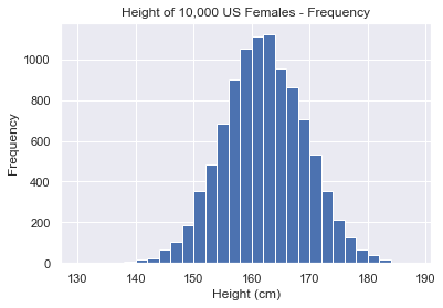
The above histogram plots the height of 10,000 US females. The x-axis is the height in cms. We have grouped the heights into ranges 2cm wide i.e. 140cm-142cm, 142cm-144cm etc. and we call these ranges bins.
Since someone can be any height, we say that height is a continuous variable. It is numeric, has order and there are an unlimited number of values. In theory, you can only plot continuous variables using a histogram. But if you are plotting discrete numerical variables e.g. the outcomes of rolling a dice, it is easier to code a histogram than a bar chart.
Note that there is no space between bins. The white lines are purely aesthetic. Plus, bins are half-open intervals. The bin 140cm-142cm is [140, 142). This means that it includes 140cm and excludes 142cm. The only exception is the final bin which is inclusive on both sides.
The y-axis is the total number of times we observed a particular height. We call this the frequency.

Histograms can also show the probability on the y-axis. The sum of the total area under a histogram is 1. We see that the probability of a US female being 158cm-160cm tall is just over 0.05. So can we say that 5% of US females we measured are this height? Unfortunately not. To get the probability of a value being in a particular bin, we calculate the area of the bar using bin_width x height. In this case, it is 2cm x 0.05 = 0.1. So 10% of women measured are 158cm-160cm tall.
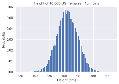
Let’s change the bin size to be 1cm.
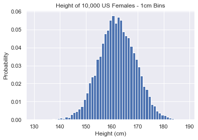
Notice that the shape of the graph is similar and the probabilities on the y-axis are the same.
Now there are 2 bars in the 158cm-160cm range. Each bar has height ~0.05. So the probability of being in each bar is:
- 158cm-159cm: 1 x 0.05 = 0.05
- 159cm-160cmL 1 x 0.05 = 0.05
Hence, the combined probability is 0.05 + 0.05 = 0.1. This is the same as above.
It’s best not to trust the probabilities on the y-axis. They will always be ‘correct’ but the actual probability of being in a particular bin is bin_width x height.
It gets more confusing if we use bins of varying size.
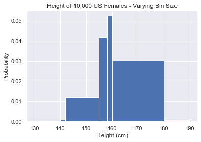
The probability of the bin 160cm-180cm is 0.03 but the actual probability of being in that bin is 20 x 0.03 = 0.6.
This is a ‘legal’ histogram. But it’s best practice to use bins of the same size. Why?
Histograms show us the distribution of our data at a glance. This is incredibly valuable. Scientists have studied many distributions extensively. If our data fits one of these distributions, we instantly know a lot about it. The shape of the above histograms is the normal distribution and you will see it everywhere.
Let’s summarize what we’ve learned about histograms. If you understand these points, plotting them will be a breeze.
A histogram is:
- A plot of one continuous variable e.g. height in cm
- We can easily see the distribution
- x-axis – continuous data grouped into bins
- No blank space between bins
- Bins do not have to have the same width (but usually do)
- y-axis – frequency or probability
- To calculate the probability of a value being in a bin, do bin_width x probability. Don’t trust the y-axis probabilities!
Now you know the theory behind histograms, let’s plot them in Python with matplotlib.pyplot.
Matplotlib Histogram – Basic Plot
First, we need some data.
I went to this site to find out the mean height and standard deviation of US females. It is common knowledge that height is normally distributed. So I used Python’s random module to create 10,000 samples
import random

# data obtained online
mean = 162
std = 7.1

# set seed so we can reproduce our results
random.seed(1)

# use list comprehension to generate 10,000 samples
us_female_heights = [random.normalvariate(mean, std) for i in range(10000)]
Optional step: Seaborn’s default plots look better than matplotlib’s, so let’s use them.
import seaborn as sns

sns.set()
The most basic histogram in in matplotlib.pyplot is really easy to do
import matplotlib.pyplot as plt

plt.hist(us_female_heights)
plt.show()
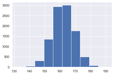
Not bad for basic settings. The general shape is clear. We see that most of the data is concentrated in the middle – 155cm-170cm. We can also see the frequency counts.
Because we know our data, we know that the x-axis is height in cm and the y-axis is frequency. But you must always label your axes. Other people don’t know what this graph is showing. Adding labels makes this clear. Write these three lines of code to give the plot a title and axis labels.
plt.hist(us_female_heights)
plt.title('Height of 10,000 US Females')
plt.xlabel('Height (cm)')
plt.ylabel('Frequency')
plt.show()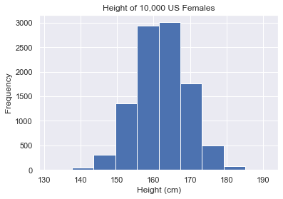
Much better!
To save space, we will not include the lines of code that label the axes. But make sure you include them.
It’s a good idea to first use the basic settings. This gives you a general overview of the data. Now let’s start modifying our histogram to extract more insights.
Matplotlib Histogram – Basic Density Plot
Knowing the frequency of observations is nice. But if we have a billion samples, it gets hard to read the y-axis. So we’d rather have probability.
In maths, a probability density function returns the probability of a continuous variable. If the variable is discrete, it’s called a probability mass function. I found this terminology very confusing when I first heard it. Check out this incredible Stack Exchange answer to understand it in more detail.
A histogram with probability on the y-axis is thus a probability density function. So we set the density keyword in plt.hist() to True.
plt.hist(us_female_heights, density=True)
plt.show()
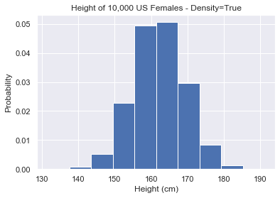
It’s very easy to swap between frequency and density plots. As density plots are more useful and easier to read, we will keep density=True from now on.
Let’s have a more detailed look at our data by changing the bin size.
Matplotlib Histogram Bins
Deciding on the optimal number of bins for a histogram is a hotly debated topic. You can affect how your data is perceived by changing this. Thus many mathematicians have created formulas to optimise bin size.
We modify the number of bins using the bins keyword in plt.hist(). It accepts an integer, list or string.
Integer Bins
To specify a particular number of bins, pass an integer to the bins keyword argument.
# 5 bins
plt.hist(us_female_heights, density=True, bins=5)
plt.show()

Setting bins to a very low value gives you a general overview of the data.
# 40 bins
plt.hist(us_female_heights, density=True, bins=40)
plt.show()
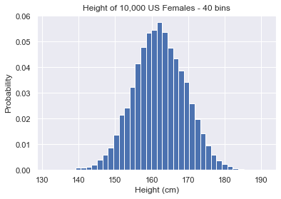
Setting bins to a high number gives you a more detailed view of the data.
Even though we set bins=40, you cannot see 40 bins on the plot. This is because the remaining bins are too small to see.
>>> min(us_female_heights)
131.67453350862354

>>> max(us_female_heights)
191.1310915602654
After checking the min/max values of our data, we see that there must be bins down to 131 and up to 192. These only contain a small number of samples so their probability is very low. Thus we cannot see them in the plot.
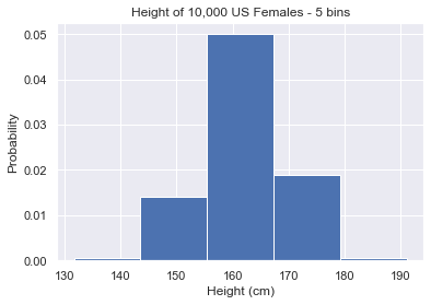
Setting bins to an integer value is a nice shortcut but we don’t recommend it. Why? Because matplotlib never chooses a nice bin width. On the bins=5 plot, the largest bin starts at ~155 and ends at ~167. This makes our histogram hard to read if we actually want to extract insights.
It’s much better to set the bin edges yourself. We do this by passing bins a list or NumPy array. If you need a refresher on the NumPy library, check out our complete NumPy tutorial that teaches you everything you need to get started with data science.
List of Bins
Once we have an idea about our data, we can set the bins manually. We humans like to work with whole numbers. So we’d like our bin edges to be whole numbers too.
An ideal situation would start at 130, end at 192 and go up in 2cm steps
ideal_bins = [130, 132, 134, ..., 192]
We use the np.arange function to create this.
ideal_bins = np.arange(130, 194, 2)
The max value is 191.1… so we want our last bin edge to be 192 (remember that the stop value is exclusive in np.arange). For a full explanation of np.arange, check out our article.
Let’s pass this to plt.hist():
plt.hist(us_female_heights, density=True, bins=ideal_bins)
plt.show()

It’s much easier to read this histogram because we know where each bin edge is.
We can make it more detailed by setting the step size to 1 in np.arange().
plt.hist(us_female_heights, density=True, bins=np.arange(130, 193, 1))
plt.show()
Nice! We now have an even more detailed overview.
To set bins of different sizes, pass a list/array with the bin edges you want.
my_bin_edges = [130, 140, 142, 155, 158, 160, 180, 190]
plt.hist(us_female_heights, density=True, bins=my_bin_edges)
plt.show()

Most of the time, you will want to plot histograms with uniform bin width. But it’s good to know how to change them to whatever you want.
String Bins
You can use several mathematical formulas to compute the optimal bin size. We will list the options available to you. If you want a more detailed explanation of each, please read the numpy docs. Each produces a good output and they are all better than matplotlib’s default settings.
- auto
- fd – Freedman Diaconis Estimator
- doane
- scott
- stone
- rice
- sturges
- sqrt
Here’s our data using bins=’auto’.

Here’s our plot using ‘scott’.
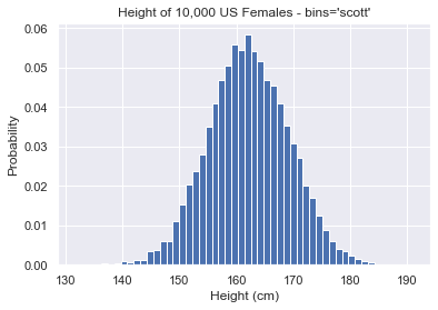
We won’t dive into the mathematics behind them or their pros and cons. Please experiment with them in your IDE. Pass each option to the bins argument to see the differences.
A big part of learning is trying new things. So for your first data analysis projects, plot your data as many ways as possible. As time goes on, you will get a ‘feel’ for which method is best.
Summary
We’ve covered the most important things you need to know to plot great histograms.
You now understand what histograms are and why they are important. You can make density plots that show the probability on the y-axis. And you can change the bin size to anything you want to better understand your data.
There is much more we can do with histograms. For example, plotting multiple histograms on top of each other, making horizontal plots or cumulative ones. But we’ll leave them for another article.
Where to Go From Here?
Enough theory. Let’s get some practice!
Coders get paid six figures and more because they can solve problems more effectively using machine intelligence and automation.
To become more successful in coding, solve more real problems for real people. That’s how you polish the skills you really need in practice. After all, what’s the use of learning theory that nobody ever needs?
You build high-value coding skills by working on practical coding projects!
Do you want to stop learning with toy projects and focus on practical code projects that earn you money and solve real problems for people?
🚀 If your answer is YES!, consider becoming a Python freelance developer! It’s the best way of approaching the task of improving your Python skills—even if you are a complete beginner.
If you just want to learn about the freelancing opportunity, feel free to watch my free webinar “How to Build Your High-Income Skill Python” and learn how I grew my coding business online and how you can, too—from the comfort of your own home.
References
- https://stackoverflow.com/questions/33203645/how-to-plot-a-histogram-using-matplotlib-in-python-with-a-list-of-data
- https://matplotlib.org/3.1.1/api/_as_gen/matplotlib.pyplot.hist.html
- https://matplotlib.org/3.1.1/gallery/statistics/hist.html
- https://keydifferences.com/difference-between-histogram-and-bar-graph.html
- https://tall.life/height-percentile-calculator-age-country/
- https://blog.finxter.com/python-random-module/
- https://math.stackexchange.com/questions/23293/probability-density-function-vs-probability-mass-function
- https://docs.scipy.org/doc/numpy/reference/generated/numpy.histogram_bin_edges.html#numpy.histogram_bin_edges