

MACD is a trend-following momentum indicator used for trading. It consists of two lines:
- The MACD line is calculated by taking the difference between short-term EMA and long-term EMA. Exponential Moving Average (EMA) assigns weights to all the values due to a given factor whereas the latest data point gets the maximum weight, and the oldest data point gets the minimum weight. The short-term EMA is usually chosen with a period of 12 units and the long-term EMA is chosen with a period of 26 units.
- The signal line is calculated using the EMA of the MACD line.
This article is based on the full trading tutorial on the Not-Satoshi blog.
Introduction
Before we begin, I would like to make a small request
- If you don’t know the basics of
binanceandpython-binanceAPI. - If you want to know how to set up the development environment, set up a
binanceaccount orbinance-testnetaccount. Then, you should please go through the previous course (Creating Your First Simple Crypto-Trading Bot with Binance API) where these are explained in detail. - Please be aware of the following note:
##################### Disclaimer!! ###################################
# The bots built here with python should be used only as a learning tool. If you choose
# to do real trading on Binance, then you have to build your own criteria
# and logic for trading. The author is not responsible for any losses
# incurred if you choose to use the code developed as part of the course on Binance.
####################################################################
Another important point:
In the algorithms we discuss, there are multiple buy/sell points to buy/sell crypto. It is up to you as to how to want to write the logic for buying and selling, e.g. In the bots we develop, buying or selling a crypto asset happens at all the buy/sell points using a for loop for each buy and sell point.
There can be multiple ways to implement the buy/sell logic, some are mentioned below
- You can keep separate loops to buy and sell and keep looping until at least one buy and one sell occurs and then break.
- You can choose to buy/sell only for a particular buy/sell signal. i.e. if market price is <= or >= a particular value from the buy/sell list. In this case, no for loop is needed here.
- You can choose to buy/sell, by placing only limit orders and not market orders with the prices from the buy/sell list.
And so on….
Let’s Begin the journey
Now that we are clear on all these things we discussed we can start with our first trading algorithm – SMA. So see you soon in our first algorithm!!
PS: Follow the videos, along with the tutorial to get a better understanding of algorithms!
Feel free to check out the full code at the Finxter GitHub repository here.
MACD Basics
To understand MACD, firstly it is important to understand Exponential Moving Average (EMA). Mathematically EMA is calculated using
EMA = [CV x Factor] + [EMAprev x (1 - Factor)]
where CV = current value of the asset
Factor = 2/(N+1), where can be the number of days or period
EMA is also called EWM (Exponential Weighted Moving) average as it assigns weights to all the values due to Factor. In the case of EMA, the latest data point gets the maximum attention, and the oldest data point gets the least attention.
MACD consists of two lines MACD line and the signal line. MACD line is calculated by taking the difference between short-term EMA and long-term EMA. The short-term EMA is usually chosen with a span or period=12 and the long-term EMA is chosen with a span or period=26. The signal line is calculated using the EMA of the MACD line.
MACD = shortEMA - longEMA
signal = EMA on MACD with a span or period = 9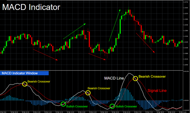
Wherever the MACD line crosses the signal line, results in buying or selling points.
If MACD cuts the signal line in the direction (see figure),
- top to the bottom -> selling point
- bottom to the top -> buying point
As the moving average here is converging or diverging from the signal line it is called Moving Average Convergence Divergence.
Bot Trading Logic
We are now clear with the basics of MACD, let’s start coding the bot. The bot will be designed in steps.
Step 1: Main Bot Skeloton
import os
from binance.client import Client
import pprint
import pandas as pd     # needs pip install
import numpy as np
import matplotlib.pyplot as plt   # needs pip install


if __name__ == "__main__":
    # passkey (saved in bashrc for linux)
    api_key = os.environ.get('BINANCE_TESTNET_KEY')
    # secret (saved in bashrc for linux)
    api_secret = os.environ.get('BINANCE_TESTNET_PASSWORD')

    client = Client(api_key, api_secret, testnet=True)
    print("Using Binance TestNet Server")

    pprint.pprint(client.get_account())
    # Change symbol here e.g. BTCUSDT, BNBBTC, ETHUSDT, NEOBTC
    symbol = 'BNBUSDT'
    main()
Import the necessary packages (binance client, pandas, NumPy, and Matplotlib).
At the start retrieve the Binance testnet API key and password using os.environ.get(). Initialize the Binance client with key, password, and testnet=true (We use only the testnet for the bot).
Any symbol can be used, here we use the ‘BNBUSDT ‘ and trigger main().
Step 2: Data Preparation
def get_data_frame():
    # valid intervals - 1m, 3m, 5m, 15m, 30m, 1h, 2h, 4h, 6h, 8h, 12h, 1d, 3d, 1w, 1M
    # request historical candle (or klines) data using timestamp from above, interval either every min, hr, day or month
    # starttime = '30 minutes ago UTC' for last 30 mins time
    # e.g. client.get_historical_klines(symbol='ETHUSDTUSDT', '1m', starttime)
    # starttime = '1 Dec, 2017', '1 Jan, 2018'  for last month of 2017
    # e.g. client.get_historical_klines(symbol='BTCUSDT', '1h', "1 Dec, 2017", "1 Jan, 2018")
    starttime = '1 day ago UTC'
    interval = '1m'
    bars = client.get_historical_klines(symbol, interval, starttime)

    for line in bars:        # Keep only first 5 columns, "date" "open" "high" "low" "close"
        del line[5:]

    df = pd.DataFrame(bars, columns=['date', 'open', 'high', 'low', 'close']) #  2 dimensional tabular data
    return df


def macd_trade_logic():
    symbol_df = get_data_frame()

def main():
    macd_trade_logic()
As a second step, define main(), macd_trade_logic() and get_data_frame(). We need historical data to start the MACD calculations.
The function get_data_frame() uses the python-binance API get_historical_klines() to get the historical data for the given interval (1min) and start time (one day ago).
Note that the interval and start time can be changed to any valid interval and start time (see comments or python-binance documentation for more details).
Finally, use the pandas DataFrame() to generate the data frame for the first five columns (date, open, high, low, and close).
Step 3: Trading Logic MACD
Calculate the short-term and long-term EMA for the close values, MACD, and signal line as described above.
def macd_trade_logic():
    symbol_df = get_data_frame()
    # calculate short and long EMA mostly using close values
    shortEMA = symbol_df['close'].ewm(span=12, adjust=False).mean()
    longEMA = symbol_df['close'].ewm(span=26, adjust=False).mean()

    # Calculate MACD and signal line
    MACD = shortEMA - longEMA
    signal = MACD.ewm(span=9, adjust=False).mean()

    symbol_df['MACD'] = MACD
    symbol_df['signal'] = signal
The EMA is calculated using the ewm (exponentially weighted moving) and mean() function of the Pandas data frame. MACD is the difference between short-term and long-term EMA and the signal line is calculated with the EMA of the MACD line.
We also add two more columns,’ MACD’ and ‘signal’.
Step 4: Trigger Buy and Sell
Whenever the MACD > signal, the moving average (EMA in this case) is either converging or diverging from the signal. This can be considered as +1, else 0. A new column ‘Trigger’ can be formed using the NumPy function where().
The np.where() function can be thought of as an if-else condition used in Python.
Further, taking the difference of two adjacent values of the ‘Trigger’ column, we get the buy and sell positions. The positions can be used to get the exact buy and sell point. The position value can be +1 for buy and -1 for sell.
    symbol_df['Trigger'] = np.where(symbol_df['MACD'] > symbol_df['signal'], 1, 0)
    symbol_df['Position'] = symbol_df['Trigger'].diff()

    # Add buy and sell columns
    symbol_df['Buy'] = np.where(symbol_df['Position'] == 1,symbol_df['close'], np.NaN )
    symbol_df['Sell'] = np.where(symbol_df['Position'] == -1,symbol_df['close'], np.NaN )
- The ‘Buy’ column is updated to a close value of the crypto asset if the ‘Position’ is 1, otherwise to NaN (Not a number).
- The ‘Sell’ column is updated to a close value of the crypto asset if the ‘Position’ is 1, otherwise to NaN (Not a number).
Finally, we have the buy/sell signals as part of MACD.
Step 5: File Output
At this stage, seeing all the columns output to a text file would be a good idea. We can use the regular file open and write functions to write to a file.
    with open('output.txt', 'w') as f:
        f.write(symbol_df.to_string())
When you run the application, you will see that the output.txt has a date, open, high, low, close, Trigger, Position, MACD, signal, Buy and Sell columns. You can observe that the date column is in Unix timestamp(ms) and not in a human-readable format. This can be changed to a human-readable format using the Pandas function to_datetime() function.
  # To print in human-readable date and time (from timestamp)
    symbol_df.set_index('date', inplace=True)
    symbol_df.index = pd.to_datetime(symbol_df.index, unit='ms')

    with open('output.txt', 'w') as f:
        f.write(symbol_df.to_string())
Step 6: Plotting
We can now visually interpret all the important symbol-related information. This can be done by plotting the graph using matplotlib and making a call to plot_graph() from macd_trade_logic()
def plot_graph(df):

    df=df.astype(float)
    df[['close', 'MACD','signal']].plot()
    plt.xlabel('Date',fontsize=18)
    plt.ylabel('Close price',fontsize=18)
    x_axis = df.index

    plt.scatter(df.index,df['Buy'], color='purple',label='Buy',  marker='^', alpha = 1) # purple = buy
    plt.scatter(df.index,df['Sell'], color='red',label='Sell',  marker='v', alpha = 1)  # red = sell

    plt.show()
Call the above function from macd_trade_logic().
plot_graph(symbol_df) # can comment this line if not needed
Step 7: Buy and Sell
Lastly, trading i.e, the actual buying or selling of the crypto, must be implemented.
def buy_or_sell(df, buy_sell_list):
    for index, value in enumerate(buy_sell_list):
        current_price = client.get_symbol_ticker(symbol =symbol)
        print(current_price['price']) # Output is in json format, only price needs to be accessed
        if value == 1.0 : # signal to buy
            if current_price['price'] < df['Buy'][index]:
                print("buy buy buy....")
                buy_order = client.order_market_buy(symbol=symbol, quantity=1)
                print(buy_order)

        elif value == -1.0: # signal to sell
            if current_price['price'] > df['Sell'][index]:
                print("sell sell sell....")
                sell_order = client.order_market_sell(symbol=symbol, quantity=1)
                print(sell_order)
        else:
            print("nothing to do...")
In the above buy_or_sell() a for loop is added to get the current price of the symbol using the get_symbol_ticker() API. The for loop iterates over the buy_sell_list.
As the buy_sell_list has either a value of ‘+1.0 ‘ for buy and ‘-1.0’ for sell, place an order on Binance to buy or sell at the market price after comparing with the current price of the symbol.
In the macd_trade_logic(), the ‘Position’ column has +1 and -1. Form a list of this column as it is much easier to iterate over the list (this is optional as you can also iterate directly over the ‘Position’ column using the data frame (df) passed as an argument)
    # get the column=Position as a list of items.
    buy_sell_list = symbol_df['Position'].tolist()

    buy_or_sell( symbol_df, buy_sell_list)
💡 Recommended: Coinbase API: Getting Historical Price for Multiple Days Made Easy
Full Code
Here’s the full code of this bot for copy&paste:
# Author: Yogesh K for finxter academy
# MACD - Moving average convergence divergence
import os
from binance.client import Client
import pprint
import pandas as pd     # needs pip install
import numpy as np
import matplotlib.pyplot as plt   # needs pip install


def get_data_frame():
    # valid intervals - 1m, 3m, 5m, 15m, 30m, 1h, 2h, 4h, 6h, 8h, 12h, 1d, 3d, 1w, 1M
    # request historical candle (or klines) data using timestamp from above, interval either every min, hr, day or month
    # starttime = '30 minutes ago UTC' for last 30 mins time
    # e.g. client.get_historical_klines(symbol='ETHUSDTUSDT', '1m', starttime)
    # starttime = '1 Dec, 2017', '1 Jan, 2018'  for last month of 2017
    # e.g. client.get_historical_klines(symbol='BTCUSDT', '1h', "1 Dec, 2017", "1 Jan, 2018")
    starttime = '1 day ago UTC'
    interval = '1m'
    bars = client.get_historical_klines(symbol, interval, starttime)

    for line in bars:        # Keep only first 5 columns, "date" "open" "high" "low" "close"
        del line[5:]

    df = pd.DataFrame(bars, columns=['date', 'open', 'high', 'low', 'close']) #  2 dimensional tabular data
    return df

def plot_graph(df):

    df=df.astype(float)
    df[['close', 'MACD','signal']].plot()
    plt.xlabel('Date',fontsize=18)
    plt.ylabel('Close price',fontsize=18)
    x_axis = df.index

    plt.scatter(df.index,df['Buy'], color='purple',label='Buy',  marker='^', alpha = 1) # purple = buy
    plt.scatter(df.index,df['Sell'], color='red',label='Sell',  marker='v', alpha = 1)  # red = sell

    plt.show()


def buy_or_sell(df, buy_sell_list):
    for index, value in enumerate(buy_sell_list):
        current_price = client.get_symbol_ticker(symbol =symbol)
        print(current_price['price']) # Output is in json format, only price needs to be accessed
        if value == 1.0 : # signal to buy (either compare with current price to buy/sell or use limit order with close price)
            if current_price['price'] < df['Buy'][index]:
                print("buy buy buy....")
                buy_order = client.order_market_buy(symbol=symbol, quantity=1)
                print(buy_order)

        elif value == -1.0: # signal to sell
            if current_price['price'] > df['Sell'][index]:
                print("sell sell sell....")
                sell_order = client.order_market_sell(symbol=symbol, quantity=1)
                print(sell_order)
        else:
            print("nothing to do...")


def macd_trade_logic():
    symbol_df = get_data_frame()

    # calculate short and long EMA mostly using close values
    shortEMA = symbol_df['close'].ewm(span=12, adjust=False).mean()
    longEMA = symbol_df['close'].ewm(span=26, adjust=False).mean()

    # Calculate MACD and signal line
    MACD = shortEMA - longEMA
    signal = MACD.ewm(span=9, adjust=False).mean()

    symbol_df['MACD'] = MACD
    symbol_df['signal'] = signal

    # To print in human readable date and time (from timestamp)
    symbol_df.set_index('date', inplace=True)
    symbol_df.index = pd.to_datetime(symbol_df.index, unit='ms') # index set to first column = date_and_time

    symbol_df['Trigger'] = np.where(symbol_df['MACD'] > symbol_df['signal'], 1, 0)
    symbol_df['Position'] = symbol_df['Trigger'].diff()

    # Add buy and sell columns
    symbol_df['Buy'] = np.where(symbol_df['Position'] == 1,symbol_df['close'], np.NaN )
    symbol_df['Sell'] = np.where(symbol_df['Position'] == -1,symbol_df['close'], np.NaN )


    with open('output.txt', 'w') as f:
        f.write(
                symbol_df.to_string()
               )


   # plot_graph(symbol_df)

    # get the column=Position as a list of items.
    buy_sell_list = symbol_df['Position'].tolist()

    buy_or_sell(symbol_df, buy_sell_list)


def main():
    macd_trade_logic()


if __name__ == "__main__":

    api_key = os.environ.get('BINANCE_TESTNET_KEY')     # passkey (saved in bashrc for linux)
    api_secret = os.environ.get('BINANCE_TESTNET_PASSWORD')  # secret (saved in bashrc for linux)

    client = Client(api_key, api_secret, testnet=True)
    print("Using Binance TestNet Server")

    pprint.pprint(client.get_account())

    symbol = 'BNBUSDT'   # Change symbol here e.g. BTCUSDT, BNBBTC, ETHUSDT, NEOBTC
    main()
Conclusions
In this post, we covered the basics of EMA (exponential moving average), the concept of MACD and signal line, and successfully designed a bot using the MACD strategy.
Running the bot will loop over all the buy and sell points, placing a market buy or sell order, similar to what we did in SMA. You can always implement your own buy_or_sell() logic based on the needs or requirements for trading.
You can also further enhance the bot by calculating the profit/loss for every buy/sell pair.
Where to Go From Here
Cryptocurrency trading is a highly sought-after skill in the 21st century. Freelancers who excel in crypto trading are paid up to $300 per hour.
If you want to learn the ins and outs of trading, check out our full course on the Finxter Computer Science academy:
🚀 Full Course: Creating Your First Simple Crypto-Trading Bot with Binance API