
This article deals with signal processing. More precisely, it shows how to smooth a data set that presents some fluctuations, in order to obtain a resulting signal that is more understandable and easier to be analyzed. In order to smooth a data set, we need to use a filter, i.e. a mathematical procedure that allows getting rid of the fluctuations generated by the intrinsic noise present in our data set. Python provides multiple filters, they differentiate based on the mathematical procedure with which they process the data.
In this article, we will see one of the most widely used filters, the so-called Savitzky-Golay filter.
To illustrate its functioning and its main parameters, we herein apply a Savitzky-Golay filter to a data set and see how the generated fitting function changes when we change some of the parameters.
Long Story Short
The Savitzky-Golay filter is a low pass filter that allows smoothing data. To use it, you should give as input parameter of the function the original noisy signal (as a one-dimensional array), set the window size, i.e. n° of points used to calculate the fit, and the order of the polynomial function used to fit the signal.
Table 1 sums up the mandatory parameters that you need to choose in order to make your Savitzky-Golay filter working properly.
| Syntax: | savgol_filter() | |
| Parameters: | x (array-like) | data to be filtered |
window length (int) | length of the filter window (odd number) | |
polyorder (int) | order of the polynomial function used to fit | |
| Return Value | y (ndarray) | the filtered data |
These are just the mandatory parameters that you need to know in order to make the function work; for further details, have a look at the official documentation.
How Does the Savitzky-Golay Filter Work?
We might be interested in using a filter, when we want to smooth our data points; that is to approximate the original function, only keeping the important features and getting rid of the meaningless fluctuations. In order to do this, successive subsets of points are fitted with a polynomial function that minimizes the fitting error.
The procedure is iterated throughout all the data points, obtaining a new series of data points fitting the original signal. If you are interested in knowing the details of the Savitzky-Golay filter, you can find a comprehensive description here.
Smoothing a data set using a Savitzky-Golay filter
Generating a noisy data set
As explained above, we use a filter whenever we are interested in removing noise and/or fluctuations from a signal. We hence start our example by generating a data set of points that contains a certain amount of noise. To do that, we use Numpy and exploit the function .random() (see the documentation).
import numpy as np

# Generating the noisy signal
x = np.linspace(0, 2*np.pi, 100)
y = np.sin(x) + np.cos(x) + np.random.random(100)
Applying the Savitzky-Golay Filter
In order to apply the Savitzky-Golay filter to our signal, we employ the function savgol_filter(), from the scipy.signal package. This function takes as first input the array containing the signal that we want to filter, the size of the “window” that is used on each iteration for smoothing the signal, and the order of the polynomial function employed for fitting the original dataset.
As we will see, the larger the window the less accurate the fitting and the smoothing procedures because we will force the function to average a greater portion of the signal. In the following code lines, we import the savgol_filter() function and apply it to the previously defined “y” array.
from scipy.signal import savgol_filter
# Savitzky-Golay filter
y_filtered = savgol_filter(y, 99, 3)
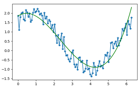
In this first example, we start with a window size of 99, which means that the function will take 99 points (almost all the points) of the initial signal to compute an average; for this reason, we do not expect to obtain good results; please also note that the order of the polynomial functions used in the fitting procedure is three.
We can now use Matplotlib to plot both the original signal and the one filtered with the Savitzky-Golay filter. If you want to become a Matplotlib expert and data visualization wizard, check out our course on the Finxter Computer Science Academy. It’s free for all premium members!
import matplotlib.pyplot as plt

# Plotting
fig = plt.figure()
ax = fig.subplots()
p = ax.plot(x, y, '-*')
p, = ax.plot(x, y_filtered, 'g')
plt.subplots_adjust(bottom=0.25)
The final result is displayed in Figure 1.
Varying the sampling window size and the order of the polynomial function
In the previous section we set the size of the sampling window to 99, which means that the filter takes as input 99 points “at a time” to compute the fitting function. Since the total number of points in the original signal is 100, the result is not really accurate (as you can also see in Figure 1). We will now create a Slider button, with which we will be able to change the size of the sampling window and see its effects immediately in the plotted graph, in order to get a better understanding of the filter working principle.
To introduce a Slider button in the plot, we exploit the Matplotlib.widget library and start by defining the properties of the button like its size and position on the matplotlib window and also the numerical values accessible through it.
# Defining the Slider button
ax_slide = plt.axes([0.25, 0.1, 0.65, 0.03]) #xposition, yposition, width and height

# Properties of the slider
win_size = Slider(ax_slide, 'Window size', valmin=5, valmax=99, valinit=99, valstep=2)
At this point, we have to define a function that will update the plot with the current value indicated by the Slider. We call the function “update”, it will get the current slider value (“win_size.val”), filter the original signal again with the new window size and plot the new filtered signal in the graph. The following code lines describe the procedure.
# Updating the plot
def update(val):
    current_v = int(win_size.val)
    new_y = savgol_filter(y, current_v, 3)
    p.set_ydata(new_y)
    fig.canvas.draw() #redraw the figure
If you are looking for a more detailed description about how to incorporate sliders and other widgets in Python, have a look at this video:
If we now plot the resulting figure, we would get the output displayed in Figure 2.
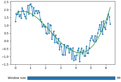
The last thing to do now, is to specify when the function “update” is triggered; we want it to be activated every time the value of the slider button gets changed.
# calling the function "update" when the value of the slider is changed
win_size.on_changed(update)
plt.show()
If we now try to reduce the size of the sampling window, we will appreciate a visible improvement in the fitting signal; this is because the Savitzky-Golay filter is called multiple times for fitting a lower amount of points at a time, hence improving the result of the fitting function. Figure 3 shows the result obtained by setting the size of the sampling window at 5 points.
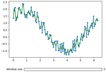
As can be seen in Figure 3, by reducing the size of the sampling window, the filtering step allows to better follow the fluctuations of the signal; in this way, the resulting signal will appear less smoothed and more detailed.
General guidelines for filtering your data
As you saw in the article, by tuning the size of the sampling window, the result of the filtering step changes quite drastically. In common practice, you should always try to keep the order of the polynomial fitting functions as low as possible in order to introduce as little distortion of the original signal as possible. Regarding the size of the sampling window, you should adjust its value in order to obtain a filtered signal which preserves all the meaningful information contained in the original one but with less noise and/or fluctuations as possible.
Keep in mind that in order to have your Savitzky-Golay filter working properly, you should always choose an odd number for the window size and the order of the polynomial function should always be a number lower than the window size.
Conclusions
In this article, we learned about the Savitzky-Golay filter, which is one of the most widely used signal filter in Python. We started by plotting a noisy signal and we then introduced the Savitzky-Golay filter with which we were able to get rid of the noise. By employing a slider button, we were also able to appreciate the variations in the fitting function as a consequence of the reduction of the sampling window size.