
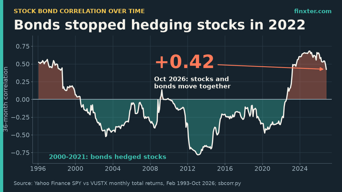
Stock bond correlation over time has flipped twice since 1993. Using monthly total returns for SPY (stocks) and Vanguard’s long-term Treasury fund VUSTX (bonds), the 36-month rolling correlation was positive in the late 1990s, negative for nearly all of 2000–2021 (as low as −0.78 in January 2013), and positive again since 2022. It peaked at +0.68 in December 2024 and sits at +0.42 as of October 2026.
That one number decides whether bonds cushion a stock crash or fall right alongside it. Below are the 405 months of data, the inflation pattern behind the flips, what it did to a 60/40 portfolio’s volatility, and a short Python script that rebuilds every number.
TL;DR
- The 36-month stock-bond correlation (SPY vs long Treasuries) is +0.42 as of October 2026, after peaking at +0.68 in December 2024.
- It was negative in 69% of windows since 1996, bottoming at −0.78 in January 2013. The 2000–2021 average was −0.29.
- In 2008, SPY lost 36.8% and long Treasuries gained 22.6%. In 2022, SPY lost 18.2% and long Treasuries lost 29.6%.
- Inflation drives it: windows with average CPI under 2.5% averaged −0.27, windows at 4%+ averaged +0.52.
- A 60/40 portfolio’s volatility rose from 8.8% to 13.3%. Short Python script included.
If you’re putting this kind of research into a guide for readers or clients, ImagineYourBook is an AI book-writing tool that turns your notes or a prompt into a full text draft with Word and EPUB export. It’s a quick way to turn a finance analysis like this one into an ebook or lead magnet.
The answer in one chart
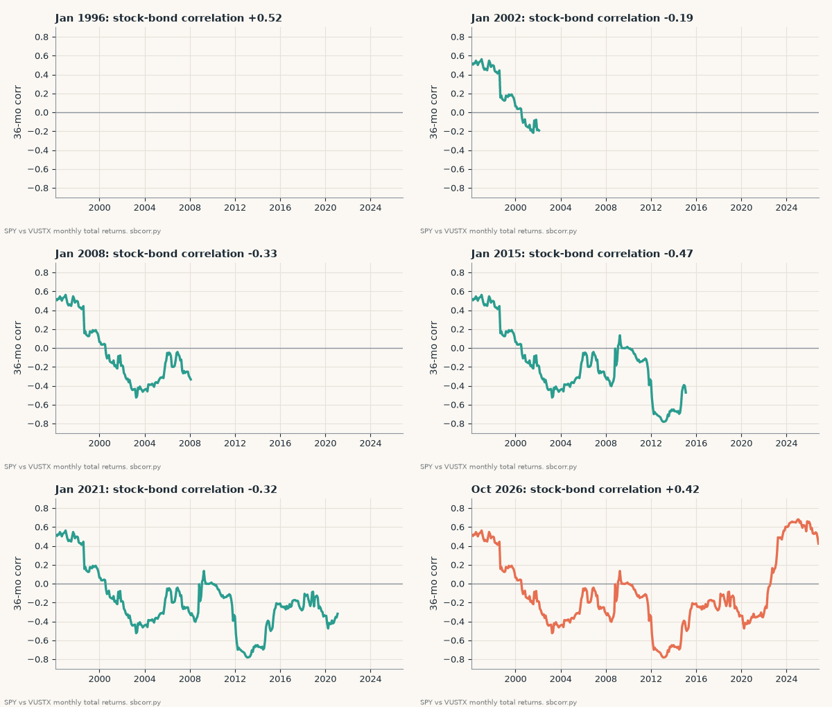
Correlation runs from −1 (bonds always move opposite to stocks) to +1 (always together). Over the whole 1993–2026 sample, the monthly correlation between SPY and long Treasuries is just −0.05, which sounds like “no relationship.” That average hides three very different regimes:
| Period | Stock-bond correlation (monthly) | Months both fell | 60/40 volatility | Stocks-alone volatility |
|---|---|---|---|---|
| Feb 1993 – Dec 1999 | +0.25 | 17% | 9.0% | 12.8% |
| Jan 2000 – Dec 2021 | −0.29 | 11% | 8.8% | 15.0% |
| Jan 2022 – Oct 2026 | +0.56 | 31% | 13.3% | 15.6% |
Out of 370 rolling 36-month windows since January 1996, 69% had a negative correlation. That’s why a whole generation of investors learned that “bonds go up when stocks go down.” The other 31% are concentrated at the two ends of the sample, and we’re living in one of them.
Total-bond funds tell the same story. VBMFX, Vanguard’s Total Bond Market Index fund, shows a 36-month correlation with SPY of +0.44 today, nearly the same as long Treasuries.
What actually happened in losing years
A correlation coefficient is abstract. Calendar-year returns aren’t. Here is every year since 1994 in which SPY lost money, next to what long Treasuries did the same year:
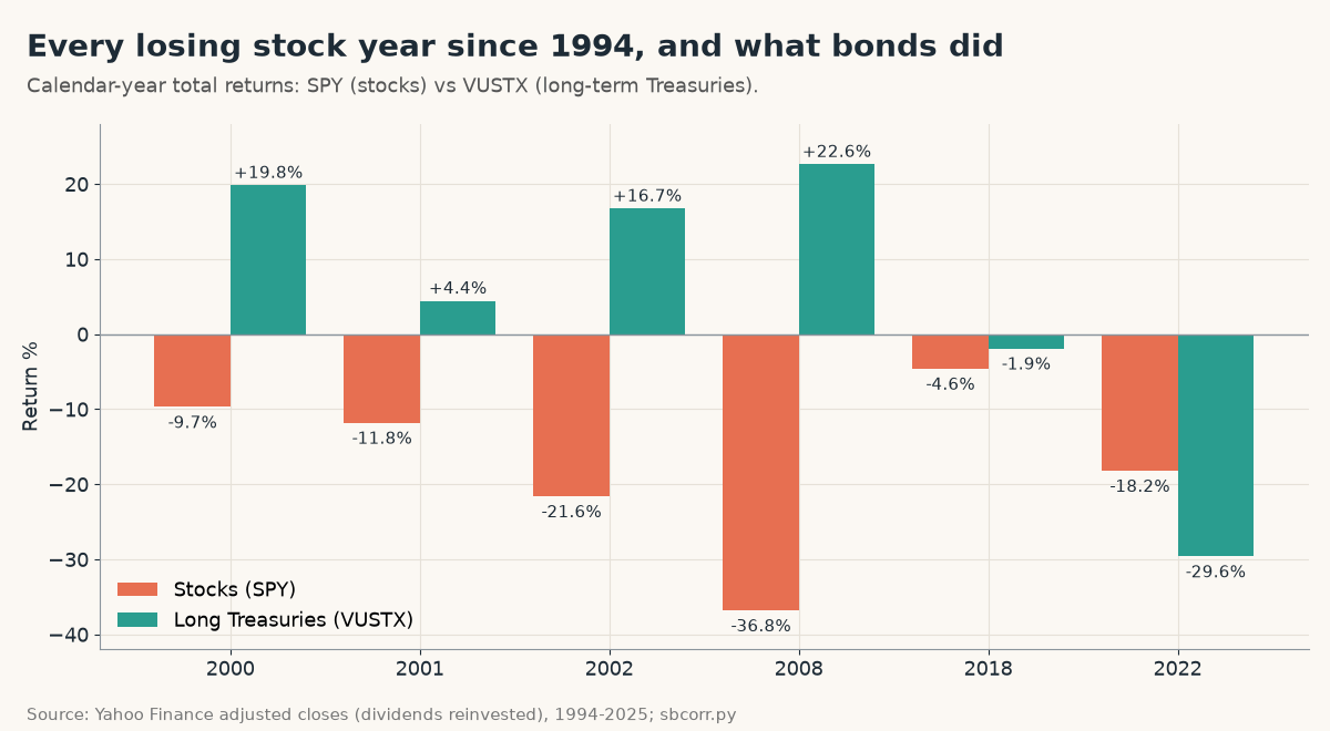
In the four big stock losses of the negative-correlation era (2000, 2001, 2002, 2008), long Treasuries gained between 4.4% and 22.6%. In 2008, SPY lost 36.8% while VUSTX gained 22.6%. That’s the hedge working exactly as advertised.
Then 2022 happened. SPY fell 18.2% and VUSTX fell 29.6%. Bonds lost more than stocks. Only one other year in the sample, 2018, saw both down, and that was a mild −4.6% and −1.9%.
The monthly data show the same shift. From 2000 to 2021, only 11% of months had both stocks and bonds negative. From January 2022 to October 2026 it was 31%, almost one month in three.
Why it flips: inflation
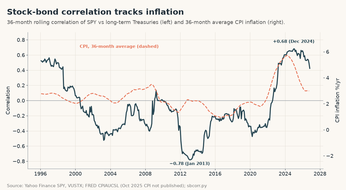
The dashed line is the 36-month average of CPI inflation from FRED. When inflation was low and stable, the correlation sat below zero. When inflation surged in 2021–2023, the correlation jumped. Across all windows, the correlation between the two lines is +0.60.
Grouping the windows by their average inflation makes the pattern blunt:
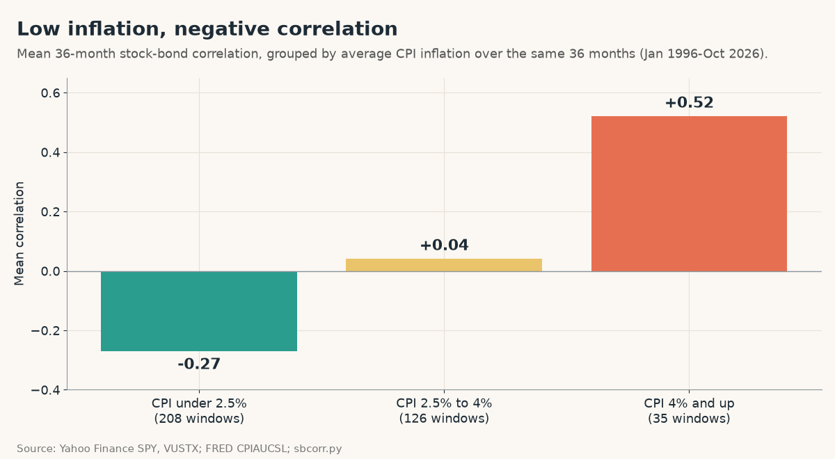
- Average CPI under 2.5%: mean stock-bond correlation −0.27 (208 windows)
- CPI 2.5% to 4%: +0.04 (126 windows)
- CPI 4% and up: +0.52 (35 windows)
This matches the research. AQR’s analysis finds that growth news pushes stocks and bonds in opposite directions while inflation news pushes them the same way, and that a simple growth-versus-inflation model explains about 70% of the long-term variation in the US stock-bond correlation. AQR also points out that the correlation was more often positive than negative from 1900 to 2000, so the 2000–2021 era, not today, is the historical outlier (AQR perspective).
Where are we now? CPI inflation was 3.7% year over year in September 2026, and the 36-month average is 3.0%. That’s the middle bucket, where history says the correlation is a coin flip. The current +0.42 is still higher than that bucket’s average, so bonds haven’t won back their hedge yet.
A data note: FRED’s CPIAUCSL series has no value for October 2025, so the 36-month averages simply skip that month.
What it costs a 60/40 portfolio
The point of holding 40% bonds is to make the ride smoother. Here’s the annualized volatility of monthly returns for stocks alone and for a 60/40 mix (60% SPY, 40% VUSTX, rebalanced monthly):
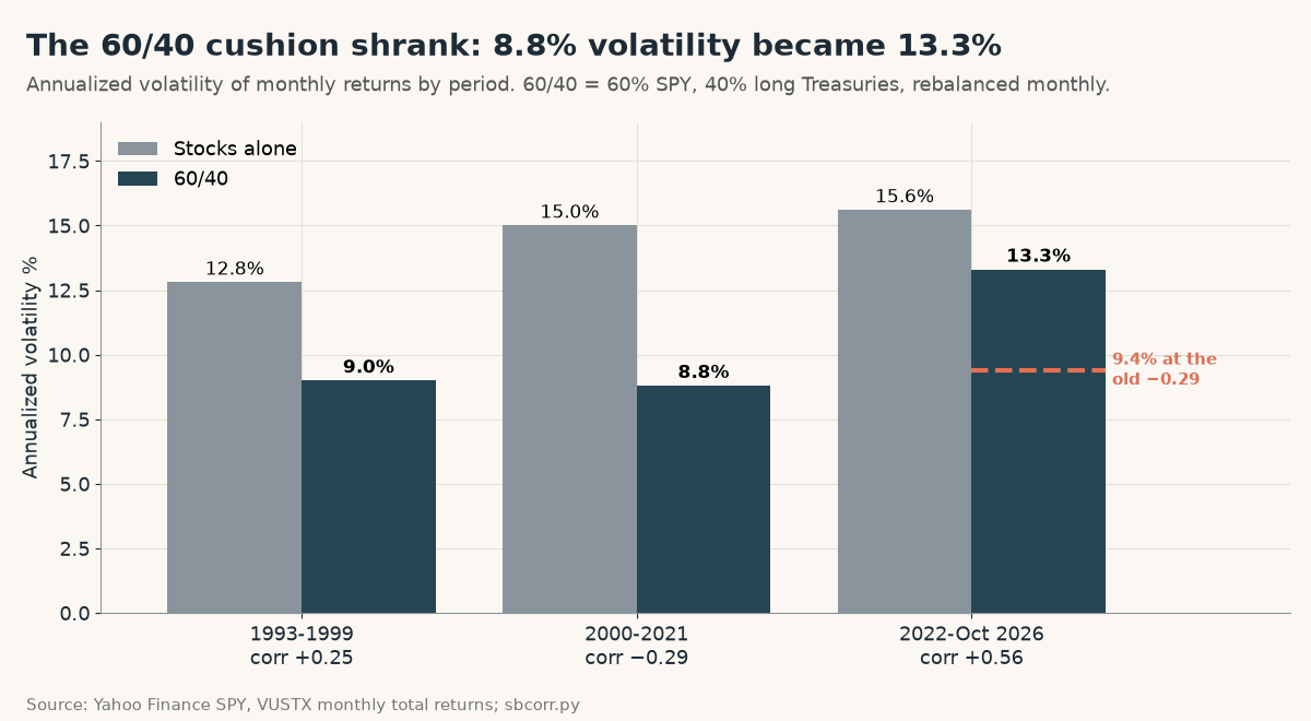
From 2000 to 2021, the 60/40 portfolio had 8.8% volatility against 15.0% for stocks alone. It removed about 41% of the swings while keeping 60% of the stock exposure. Since 2022, the same mix has run at 13.3% against 15.6% for stocks. It removed only about 15%.
How much of that is the correlation flip and how much is just jumpier bonds (14.0% volatility since 2022, up from 10.9%)? Plug the 2022–2026 volatilities into the 60/40 formula but keep the old −0.29 correlation, and you get 9.4%. So of the 4.5-point rise in 60/40 volatility, about 3.9 points come from the correlation turning positive. The bonds themselves got riskier, but losing the hedge did most of the damage.
The rule to remember: bonds hedge stocks when growth fears dominate, and fall with stocks when inflation fears dominate. Since 2022, a 60/40 portfolio has carried about 85% of the volatility of stocks alone, up from 59% in 2000–2021.
If you want to see how this plays out in drawdowns, our 60/40 portfolio max drawdown post has the peak-to-trough numbers, and how often to rebalance covers the rebalancing side. And if you’re retiring into a positive-correlation regime, the sequence of returns risk example shows why the first few years matter most.
The Python script
The script below downloads nothing by itself. Fetch daily adjusted closes once with yfinance (for example yf.download("SPY", start="1990-01-01", auto_adjust=True).to_pickle("src/SPY.pkl"), and the same for VUSTX and VBMFX), and save FRED’s CPIAUCSL CSV to src/. Then run it:
"""Stock bond correlation over time: SPY vs long-term Treasuries (VUSTX), monthly total returns.
Data: Yahoo Finance adjusted closes via yfinance (dividends reinvested), Feb 1993 - Oct 2026."""
import pandas as pd

def monthly(t, pkl="src/{}.pkl"):
    px = pd.read_pickle(pkl.format(t))["Close"].squeeze()
    return px.resample("ME").last().pct_change().dropna()

def data():
    df = pd.concat({"stocks": monthly("SPY"), "bonds": monthly("VUSTX"), "total": monthly("VBMFX")}, axis=1, sort=True).dropna()
    return df.loc["1993-02":"2026-10"]

def rolling_corr(df, n=36, b="bonds"):
    return df["stocks"].rolling(n).corr(df[b]).dropna()

def cpi_yoy(csv="src/CPIAUCSL.csv"):
    c = pd.read_csv(csv, index_col=0, parse_dates=True).squeeze()
    c.index = c.index + pd.offsets.MonthEnd(0)
    return c.pct_change(12).dropna()

def vol_6040(vs, vb, rho, w=0.6):
    return (w*w*vs*vs + (1-w)**2*vb*vb + 2*w*(1-w)*rho*vs*vb) ** 0.5

def regime_stats(df, start, end, w=0.6):
    d = df.loc[start:end]; p = w * d["stocks"] + (1 - w) * d["bonds"]
    vol = lambda s: s.std() * 12 ** 0.5
    return dict(corr=d["stocks"].corr(d["bonds"]), corr_agg=d["stocks"].corr(d["total"]), vol_s=vol(d["stocks"]), vol_b=vol(d["bonds"]), vol_p=vol(p),
                months=len(d), both_down=((d["stocks"] < 0) & (d["bonds"] < 0)).mean())

if __name__ == "__main__":
    df = data(); rc = rolling_corr(df); ra = rolling_corr(df, b="total")
    print(f"months {len(df)}: {df.index[0]:%Y-%m} to {df.index[-1]:%Y-%m}")
    print(f"full-period corr stocks/long Treasuries {df.stocks.corr(df.bonds):+.2f}, stocks/total bond {df.stocks.corr(df.total):+.2f}")
    print(f"36m rolling: latest {rc.iloc[-1]:+.2f} ({rc.index[-1]:%Y-%m}); min {rc.min():+.2f} ({rc.idxmin():%Y-%m}); max {rc.max():+.2f} ({rc.idxmax():%Y-%m})")
    print(f"share of 36m windows below zero: {(rc < 0).mean():.0%}; latest total-bond 36m {ra.iloc[-1]:+.2f}")
    for a, b in (("1993-02", "1999-12"), ("2000-01", "2021-12"), ("2022-01", "2026-10")):
        s = regime_stats(df, a, b)
        print(f"{a}..{b}: corr {s['corr']:+.2f} (agg {s['corr_agg']:+.2f}), vol stocks {s['vol_s']:.1%} bonds {s['vol_b']:.1%} 60/40 {s['vol_p']:.1%}, both-down months {s['both_down']:.0%}")
    y = (1 + df).groupby(df.index.year).prod() - 1; y = y.loc[1994:2025]
    both = y[(y.stocks < 0) & (y.bonds < 0)]
    print("calendar years both down (1994-2025):", ", ".join(f"{i}: stocks {r.stocks:+.1%} bonds {r.bonds:+.1%}" for i, r in both.iterrows()))
    neg = y[y.stocks < 0]
    print("stock down years:", ", ".join(f"{i}: {r.stocks:+.1%}/{r.bonds:+.1%}" for i, r in neg.iterrows()))
    s22 = regime_stats(df, "2022-01", "2026-10"); s00 = regime_stats(df, "2000-01", "2021-12")
    print(f"2022-26 60/40 vol if corr had stayed {s00['corr']:+.2f}: {vol_6040(s22['vol_s'], s22['vol_b'], s00['corr']):.1%} (actual {s22['vol_p']:.1%})")
    inf = cpi_yoy().reindex(rc.index); inf36 = cpi_yoy().resample("ME").last().rolling(36, min_periods=33).mean().reindex(rc.index)
    print(f"corr of 36m stock-bond correlation with 36m avg CPI inflation: {rc.corr(inf36):+.2f}")
    for lo, hi in ((0, 0.025), (0.025, 0.04), (0.04, 0.2)):
        m = (inf36 >= lo) & (inf36 < hi); print(f"  avg CPI {lo:.1%}-{hi:.1%}: {m.sum()} windows, mean corr {rc[m].mean():+.2f}")
    print(f"latest CPI YoY {cpi_yoy().iloc[-1]:.1%} ({cpi_yoy().index[-1]:%Y-%m}), latest 36m avg {inf36.dropna().iloc[-1]:.1%} ({inf36.dropna().index[-1]:%Y-%m})")
    for d in ("2008-12", "2013-01", "2019-12", "2021-12", "2024-12"):
        print(f"  36m corr at {d}: {rc.loc[d].iloc[0]:+.2f}")
Output (data through October 2026):
months 405: 1993-02 to 2026-10
full-period corr stocks/long Treasuries -0.05, stocks/total bond +0.16
36m rolling: latest +0.42 (2026-10); min -0.78 (2013-01); max +0.68 (2024-12)
share of 36m windows below zero: 69%; latest total-bond 36m +0.44
1993-02..1999-12: corr +0.25 (agg +0.32), vol stocks 12.8% bonds 7.9% 60/40 9.0%, both-down months 17%
2000-01..2021-12: corr -0.29 (agg -0.07), vol stocks 15.0% bonds 10.9% 60/40 8.8%, both-down months 11%
2022-01..2026-10: corr +0.56 (agg +0.61), vol stocks 15.6% bonds 14.0% 60/40 13.3%, both-down months 31%
calendar years both down (1994-2025): 2018: stocks -4.6% bonds -1.9%, 2022: stocks -18.2% bonds -29.6%
stock down years: 2000: -9.7%/+19.8%, 2001: -11.8%/+4.4%, 2002: -21.6%/+16.7%, 2008: -36.8%/+22.6%, 2018: -4.6%/-1.9%, 2022: -18.2%/-29.6%
2022-26 60/40 vol if corr had stayed -0.29: 9.4% (actual 13.3%)
corr of 36m stock-bond correlation with 36m avg CPI inflation: +0.60
  avg CPI 0.0%-2.5%: 208 windows, mean corr -0.27
  avg CPI 2.5%-4.0%: 126 windows, mean corr +0.04
  avg CPI 4.0%-20.0%: 35 windows, mean corr +0.52
latest CPI YoY 3.7% (2026-09), latest 36m avg 3.0% (2026-09)
  36m corr at 2008-12: -0.14
  36m corr at 2013-01: -0.78
  36m corr at 2019-12: -0.34
  36m corr at 2021-12: -0.32
  36m corr at 2024-12: +0.68
A few choices worth knowing about. Monthly returns smooth out daily noise. Thirty-six months is a common window, and a 12-month window swings much harder, while AQR uses 10-year windows in its research. Adjusted closes include dividends and bond interest, so these are total returns. And VUSTX is a long-duration fund, so it reacts more to rate moves than a short-term bond fund would.
To track your own mix of stock and bond ETFs against the S&P 500 without handing your data to anyone, PortfolioTracker24 is a free tracker that runs in your browser, with no account, no broker connection, and Excel backups.
What to do with this
- Check the regime before trusting the hedge. Re-run the script every few months. A 36-month correlation above zero means your bonds are not a crash hedge right now.
- Watch inflation, not the headlines. The windows with average CPI under 2.5% averaged a −0.27 correlation. Inflation stabilizing below that level is the clearest historical sign that the old hedge returns.
- Don’t assume more stocks is the fix. AQR argues that a positive correlation is a bad reason to take more equity risk, because you’re adding exposure to the same shocks that already hit both assets.
- Hold cash for spending needs. In 2022 both legs fell together. A cash or short-term bucket for near-term withdrawals doesn’t depend on any correlation.
| Finding | 2000–2021 | Since 2022 | What it means |
|---|---|---|---|
| Stock-bond correlation | −0.29 | +0.56 (+0.42 latest 36 mo) | Bonds no longer offset stock losses reliably |
| Months with both down | 11% | 31% | Nearly one month in three hits both legs |
| Worst stock year | 2008: SPY −36.8%, VUSTX +22.6% | 2022: SPY −18.2%, VUSTX −29.6% | The hedge flipped in the crash that mattered |
| 60/40 volatility | 8.8% | 13.3% (9.4% at the old correlation) | About 3.9 points of the rise came from the correlation |
| Inflation link | CPI avg under 2.5%: −0.27 | CPI avg 4%+: +0.52 | Watch inflation to judge the hedge |
FAQ
What is the stock bond correlation right now?
Using monthly SPY and long-term Treasury (VUSTX) returns, the 36-month correlation is +0.42 as of October 2026. It peaked at +0.68 in December 2024 and has been positive since 2022.
Has the stock bond correlation always been negative?
No. It was +0.25 from 1993 to 1999 and −0.29 from 2000 to 2021. AQR notes it was more often positive than negative from 1900 to 2000, so the negative era was the exception.
Why did stocks and bonds fall together in 2022?
Inflation. Rising inflation and interest rates hurt both. SPY lost 18.2% and long Treasuries lost 29.6%. Windows with average CPI of 4% or more had a mean correlation of +0.52.
Do bonds still diversify a stock portfolio?
Less than before. A 60/40 mix had 8.8% volatility versus 15.0% for stocks in 2000–2021, but 13.3% versus 15.6% since 2022. About 3.9 points of that rise came from the correlation turning positive.
How do I calculate stock bond correlation in Python?
Resample daily adjusted closes to month-end, take pct_change() for monthly returns, then use stocks.rolling(36).corr(bonds) in pandas. The script in this article does that for SPY and VUSTX.
The takeaway
Stock bond correlation over time isn’t a constant you can set and forget. It was +0.25 in the 1990s, −0.29 from 2000 to 2021, and +0.56 since 2022, and it tracks inflation closely. Today’s +0.42 means a 60/40 portfolio is behaving more like 85% of a stock portfolio than the 59% many investors got used to. The script above lets you check where the regime stands in seconds.
If you’ve built up investing knowledge like this and want to share it as a guide, course companion, or newsletter lead magnet, ImagineYourBook can turn your notes into a full book draft. Plans start with a 7-day free trial, and the Author plan is $24.99 a month after that.
Sources (checked November 10, 2026): Yahoo Finance: SPY history · Yahoo Finance: VUSTX history · Yahoo Finance: VBMFX history · yfinance on GitHub · FRED: CPIAUCSL consumer price index · AQR: A Changing Stock-Bond Correlation · AQR: A positive stock-bond correlation is a terrible reason to add equity risk · ImagineYourBook pricing and trial terms. Script: sbcorr.py (shown above). Past correlations don’t predict future ones. Not investment advice.